Bivariate Exponential Integrals and Edge-Bicolored Graphs

On this page, we provide an implementation in Julia of our algorithm presented in Section 4 to compute the weighted number of bicolored graphs with fixed Euler characteristic and vertex incidence structure. Then we explain how we can use our algorithm to infer an asymptotic formula for the weighted number of such graphs numerically and compare it to our theoretical result in Theorem 5.4.
In order to install the correct dependencies you should download the two files Manifest.toml and Project.toml and save them in the directory from which you are running Julia. Then enter Pkg mode (type ] in Julia) and type instantiate to install all necessary dependencies. You can either execute the code-blocks in the following one-by-one or download the complete .jl file here: bicolored.jl. To load the packages we require for our implementation type
using HomotopyContinuation
using LinearAlgebra
using Plots
using LaTeXStrings
using AMRVW
Computing the coefficients \(A_n\) efficiently
We describe our implementation of the algorithm proposed in Section 4 of our paper to compute the coefficient \(A_n\) in the generating function of bicolored graphs
We first need to set the BigFloat precision high enough so we are able to compute \(A_n\) for large \(n\):
setprecision(BigFloat, 1000; base=10)
Here is a function computing the double factorial appearing in our algorithm.
function dfactorial(n)
    if n <= 0
        return 1
    elseif n % 2 == 0
        return 0
    else
        return BigInt(n*dfactorial(n-2))
    end
end
We need to define the following variables:
@var x,y,a,u
Here, \(a\) serves as a parameter (in our paper called \(\lambda\)) and \(u\) is an auxiliary variable. The following function then implements the algorithm from Proposition 4.1.
function get_n_coeff(n, V; vars=variables(V))
    Vu = 1/u^2 * subs(V, vars => u*vars)

    d = degree(Vu, [u])
    Fs = deleteat!(reverse(coeffs_as_dense_poly(u*differentiate(Vu, u), [u], d)), 1)
    Qs = Vector{Any}([Rational{BigInt}(1)])
    for i in 1:2*n
        push!(Qs, expand(1//i * sum(Fs[j]*Qs[length(Qs) - j + 1] for j in 1:min(length(Fs), length(Qs)))))
    end

    (M, c) = exponents_coefficients(Qs[2*n + 1], vars)
    nth_coeff = Rational{BigInt}(0)
    for i in 1:size(M,2)
        m = M[:, i]
        nth_coeff += prod(dfactorial(l - 1) for l in m) * c[i]
    end
    return nth_coeff
end
We can then, e.g., recover the expansion depicted in the figure above: it shows all 4-regular graphs with Euler characteristic \(-2\) where each vertex has an even number of edges of each color. Every yellow edge is weighted by a parameter \(\lambda\).
V = x^4//24 + a^2*y^4//24 + a*x^2*y^2//4
get_n_coeff(2, V, vars=[x,y])
The code returns
Note that if \(V\) contains parameters (as above) one needs to specify in the function what the variables of \(V\) are (e.g., vars=[x,y]).
Inferring the asymptotic formula for \(A_n\)
We now describe how to use the algorithm above to infer an asymptotic formula for \(A_n\) in the large \(n\) limit and compare it with our formula provided in Theorem 5.4. First we need the following auxiliary function to substitute BigFloat values for the parameters \(\lambda\) in the expansion coefficient \(A_n\).
function big_evaluate(c, paramvals; params=[a])
    (expos, coeffs) = exponents_coefficients(c, params)
    return sum(coeffs[i] * (prod(map((i,j) -> big(i)^j, paramvals, expos[i]))) for i in 1:length(expos))
end
We make the ansatz
Dividing by \(\Gamma(n)\) and taking the logarithm of the above expression yields
Here, lower order terms in the \(\log\left(\frac{A_n}{\Gamma(n)}\right)\) expansion are of the form
We now define the matrix \(M\) via
Here, \(n_i\) and \(r\) should be chosen sufficiently large, e.g., \(n_i \geq 100\) and \(r \geq 10\). Moreover, one should choose \(n_i\) in a way such that \(A_n\neq 0\): if \(V\) is homogeneous of degree \(k\) then \(\frac{2n}{k-2}\) and \(\frac{nk}{k-2}\) need to be integers (see Proposition 5.1 and the discussion before). One then solves the linear system
for an explicit choice of \(\lambda\) numerically to obtain a solution
The following function implements this procedure and returns the triple \((\alpha(\lambda),\beta(\lambda),c(\lambda))\) for a specific choice of \(\lambda\) (called aval in the code).
function get_asymp_expansion_params_hom(V, aval; r=10, n=150, digits=10)
    k = degree(V, [x,y])
    n = Int(floor((n-r)/(k-2)))
    ag = [log(big_evaluate(get_n_coeff((k-2)*(n-i), V, vars=[x,y]), [aval])/factorial((k-2)*big(n-i)-1)) for i in 0:r]
    M = transpose(hcat([vcat([(k-2)*big(n-i), log((k-2)*big(n-i)), big(1)], [1/((k-2)*big(n-i))^(j) for j in 1:r-2]) for i in 0:r]...))
    X = Float64.(round.(M \ ag, digits=digits))
    return [exp(X[1]), X[2], exp(X[3])]
end
In Example 5.3 we show that for \(V(x,y) = \frac{x^4}{4!} + \lambda \frac{x^2 y^2}{4} + \lambda^2 \frac{y^4}{4!}\) and \(\lambda \in (0, \frac{1}{3})\) we have
We can check this numerically via the function above: the following code creates a plot comparing the true value of \(c(\lambda)\) with the numerically computed value for \(\lambda\in\left\{ 0, \frac{1}{60},\frac{2}{60},\dots, \frac{20}{60} \right\}\).
avalues = vcat([i/60 for i in 0:20])
V = x^4//24 + a^2*y^4//24 + a*x^2*y^2//4
params = [get_asymp_expansion_params_hom(V, av, n=100) for av in avalues]
plot(avalues, [param[3] for param in params], linewidth=4, linecolor=colorant"rgb(68,170,153)", label="numerical", dpi=800, xticks=([0,0.1,0.2,0.3], [L"0", L"0.1", L"0.2", L"0.3"]), yticks=([0.2,0.4,0.6,0.8,1.0], [L"0.2", L"0.4", L"0.6", L"0.8", L"1.0"]))
plot!(avalues, [1/pi * sqrt(1/(2-6*av)) for av in avalues], linewidth=4, linecolor=colorant"rgba(187,85,102,0.5)", label="true", dpi=800)
xlabel!(L"\lambda", dpi=800)
ylabel!(L"c(\lambda)", dpi=800)
This produces the following plot:

The numerics are very accurate except near the phase transition at \(\lambda=\frac{1}{3}\).
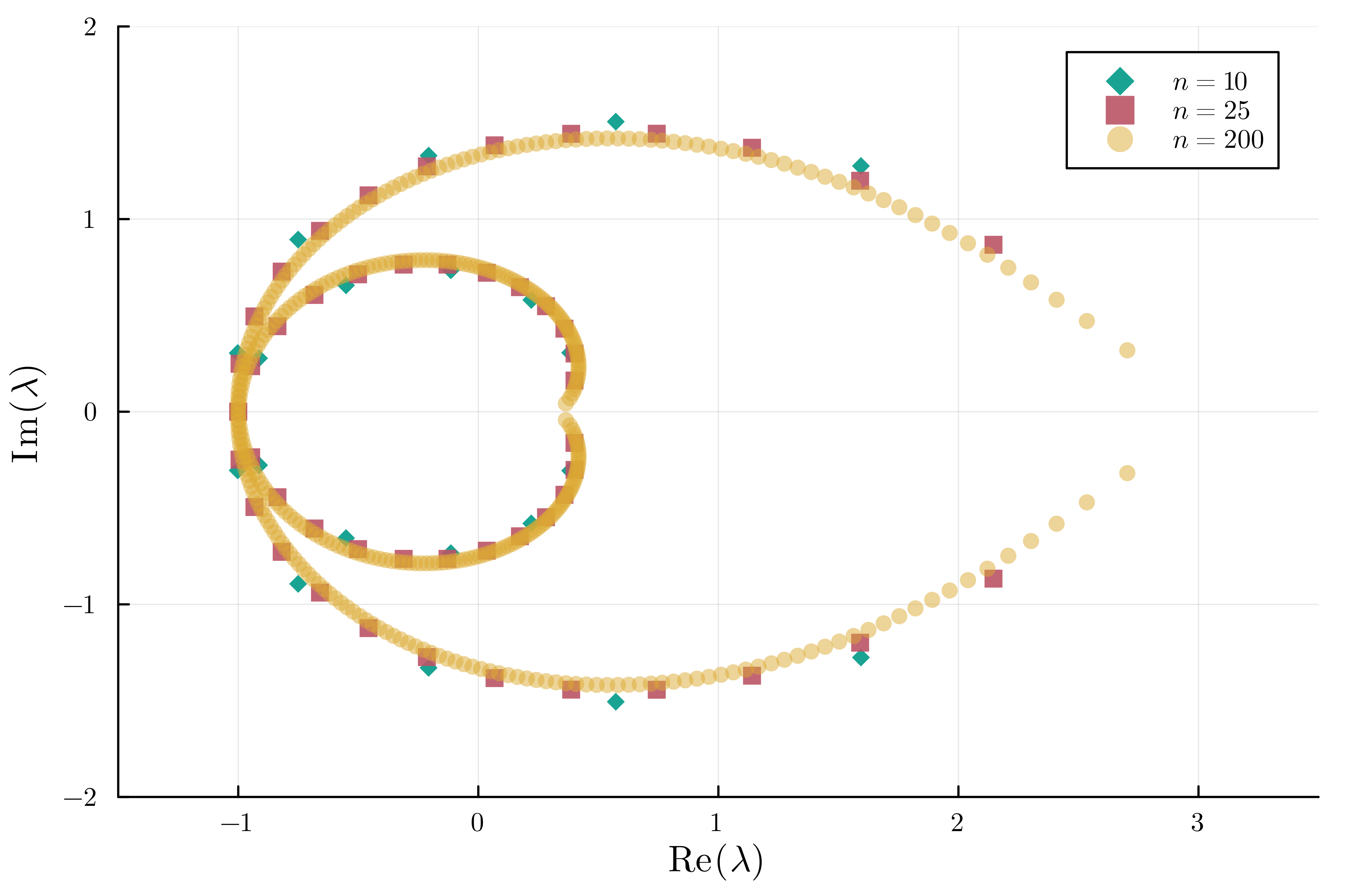
In the spirit of Lee-Yang theory, the two phase transitions \(\lambda=\frac{1}{3},3\) in the running example can be detected also by looking at the asymptotic behavior of the roots of \(A_n(\lambda)\) as \(n\to \infty\). We can compute this for the Ising model via the following code, making use of the AMRVW package to compute zeros of high-degree univariate polynomials quickly.
V = x^4//24 + a^2*y^4//24 + a*x^2*y^2//4
cfs = [coefficients(get_n_coeff(i, V, vars=[x,y]), a) for i in [10, 25, 200]]
roots = [AMRVW.roots(float.(cf)) for cf in cfs]
scatter(roots[1], xlims=(-1.5, 3.5), ylims=(-2,2), label=L"n=10", markershape=:diamond, markercolor=colorant"rgb(0,153,136)", markeralpha=0.9, markerstrokewidth=0, dpi=800)
scatter!(roots[2], label=L"n=25", markershape=:square, markercolor=colorant"rgb(187,85,102)", markeralpha=0.9, markerstrokewidth=0, dpi=800)
scatter!(roots[3], label=L"n=200", markershape=:circle, markercolor=colorant"rgb(221,170,51)", markeralpha=0.5, markerstrokewidth=0, dpi=800)
xlabel!(L"\mathrm{Re}\,(\lambda)")
ylabel!(L"\mathrm{Im}\,(\lambda)")
xticks!([-1,0,1,2,3], [L"-1", L"0", L"1", L"2", L"3"])
yticks!([-2,-1,0,1,2], [L"-2", L"-1", L"0", L"1", L"2"])
savefig("plot_zeros.png")
This produces the following plot:

Numerical Evidence for Conjecture 5.9
With a slight modification the code to infer the asymptotic formula also works for inhomogeneous polynomials. This is done via the following function.
function get_asymp_expansion_params_inhom(V, aval; r=10, n=150, digits=10)
    ag = [log(big_evaluate(get_n_coeff(n-i, V, vars=[x,y]), [aval])/factorial(big(n-i)-1)) for i in 0:r]
    M = transpose(hcat([vcat([big(n-i), log(big(n-i)), big(1)], [1/(big(n-i))^(j) for j in 1:r-2]) for i in 0:r]...))
    X = Float64.(round.(M \ ag, digits=digits))
    return [exp(X[1]), X[2], exp(X[3])]
end
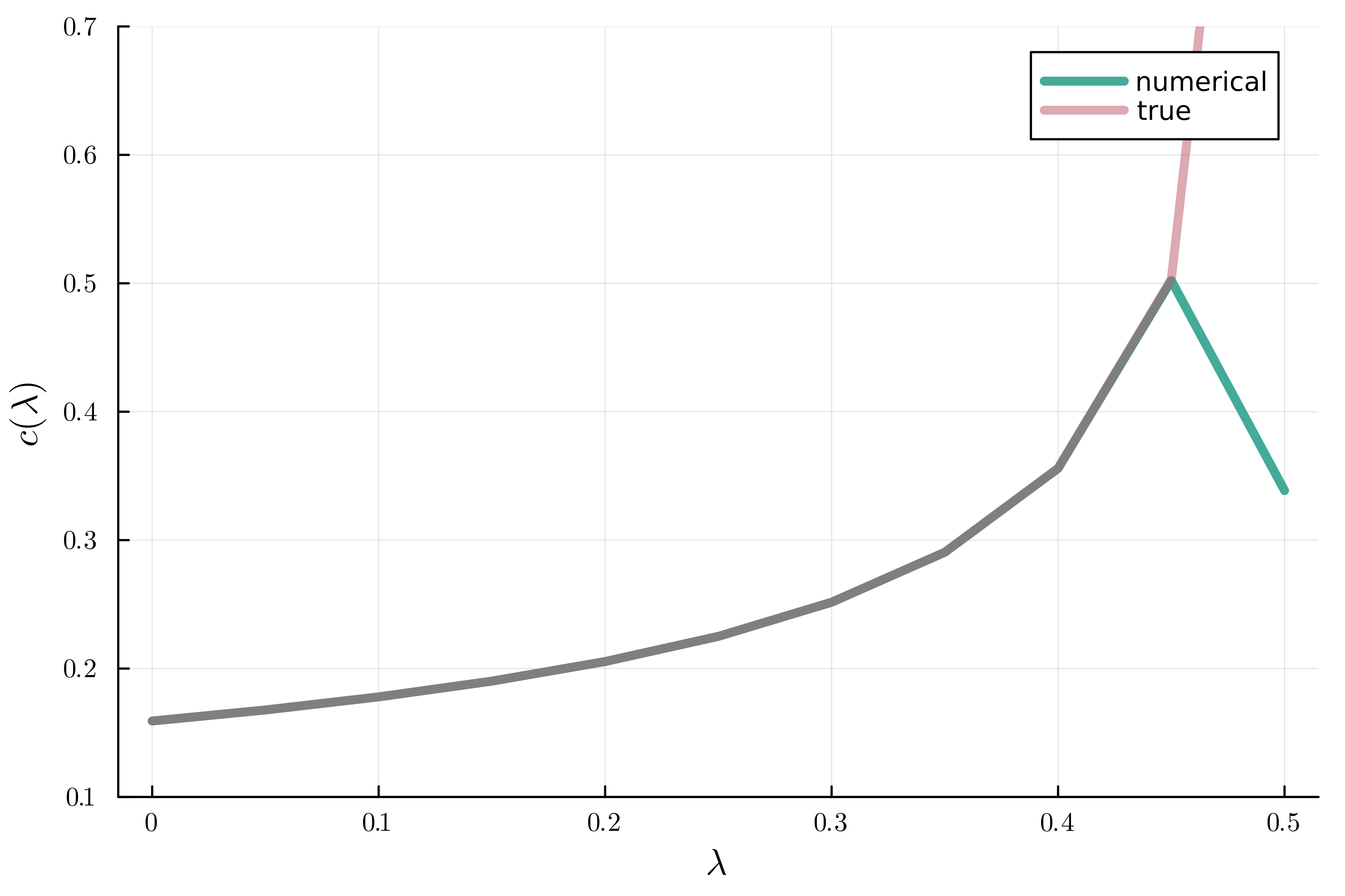
With the help of this function we can find evidence for our Conjecture 5.9. For example, for \(V(x,y) = \frac{x^3}{3!} + \lambda \frac{x y^2}{2} + \lambda^2 \frac{y^4}{4!}\) we expect \(c(\lambda) = \frac{1}{2\pi\sqrt{1-2\lambda}}\) for \(\lambda\in (0,\frac{1}{2})\). We compute \(c(\lambda)\) numerically for \(\lambda\in\{0, \frac{1}{20}, \frac{2}{20}, \dots, \frac{10}{20}\}\) using the coefficient \(A_{50}\) via the following code.
V = x^3//6 + a^2*y^4//24 + a*x*y^2//2
avalues = vcat([i/20 for i in 0:10])
params = [get_asymp_expansion_params_inhom(V, av, n=50) for av in avalues]
plot(avalues, [param[3] for param in params], linewidth=4, linecolor=colorant"rgb(68,170,153)", label="numerical", dpi=800, ylims=(0.1,0.7), xticks=([0,0.1,0.2,0.3,0.4,0.5], [L"0", L"0.1", L"0.2", L"0.3", L"0.4", L"0.5"]), yticks=([0.1,0.2,0.3,0.4,0.5,0.6,0.7], [L"0.1", L"0.2", L"0.3", L"0.4", L"0.5", L"0.6", L"0.7"]))
plot!(vcat(avalues[1:10], [0.49]), [1/(2*pi*sqrt(1-2*av)) for av in vcat(avalues[1:10], [0.49])], linewidth=4, linecolor=colorant"rgba(187,85,102,0.5)", label="true", dpi=800)
xlabel!(L"\lambda", dpi=800)
ylabel!(L"c(\lambda)", dpi=800)
savefig("plot_c_inhom.png")
This produces the following plot:

Indeed, the numerics seem to match our conjecture (again, the numerics break down near the phase transition at \(\lambda=\frac{1}{2}\)). Note that it takes much longer to compute the coefficients \(A_n\) for inhomogeneous \(V\) due to internal handling of the polynomials in HomotopyContinuation.
Project page created: 25/09/2024.
Project contributors: Michael Borinsky, Chiara Meroni, Maximilian Wiesmann.
Corresponding author of this page: Maximilian Wiesmann, wiesmann@mis.mpg.de.
Code written by: Michael Borinsky, Chiara Meroni, Maximilian Wiesmann.
Software used: Julia (Version 1.9.1).
System setup used: MacBook Pro with macOS Monterey 12.5, Processor Apple M1 Pro, Memory 16 GB LPDDR5.
License for code of this project page: MIT License (https://spdx.org/licenses/MIT.html).
License for all other content of this project page (text, images, …): CC BY 4.0 (https://creativecommons.org/licenses/by/4.0/).
Last updated 27/09/2024.