No eleventh conditional Ingleton inequality
ABSTRACT: A rational probability distribution on four binary random variables \(X, Y, Z, U\) is constructed which satisfies the conditional independence relations \(X ⫫ Y\), \(X ⫫ Z \mid U\), \(Y ⫫ U \mid Z\) and \(Z ⫫ U \mid XY\) but whose entropy vector violates the Ingleton inequality. This settles a recent question of Studený (IEEE Trans. Inf. Theory vol. 67, no. 11) and shows that there are, up to symmetry, precisely ten inclusion-minimal sets of conditional independence assumptions on four discrete random variables which make the Ingleton inequality hold. The last case in the classification of which of these inequalities are essentially conditional is also settled.
Completeness of the classification
Section 2.3 in the paper describes a method based on SAT solvers to quickly verify Studený’s claim that the three sets of CI assumptions for a (CI-type) conditional Ingleton inequality which are refuted in the paper are really the only ones left. This algorithm is implemented in the Perl script
The program writes a boolean formula in the standard DIMACS CNF format which can be solved by the SAT solver \(\verb|CaDiCaL|\), for example:
perl cases.pl | cadical
s UNSATISFIABLE
The formula describes all sets of CI assumptions which are covered neither by a proof nor a counterexample and includes the counterexample from the paper. Hence, the unsatisfiability of the formula shows that no set of CI assumptions is not covered and the classification is complete.
The counterexample from the paper can be excluded by using the --no-paper
option. Then, using an AllSAT solver such as Toda and Soh’s \(\verb|nbc_minisat_all|\)
all uncovered cases can be enumerated:
perl cases.pl --no-paper | nbc_minisat_all
-1 -2 -3 -4 -5 -6 7 -8 -9 -10 -11 -12 -13 -14 -15 -16 -17 -18 19 -20 -21 -22 -23 24 0
-1 -2 -3 -4 -5 -6 -7 -8 -9 -10 11 -12 -13 -14 15 -16 -17 -18 -19 -20 -21 -22 -23 24 0
1 -2 -3 -4 -5 -6 7 -8 -9 -10 -11 -12 -13 -14 -15 -16 -17 -18 19 -20 -21 -22 -23 -24 0
1 -2 -3 -4 -5 -6 7 -8 -9 -10 -11 -12 -13 -14 -15 -16 -17 -18 19 -20 -21 -22 -23 24 0
1 -2 -3 -4 -5 -6 -7 -8 -9 -10 11 -12 -13 -14 15 -16 -17 -18 -19 -20 -21 -22 -23 -24 0
1 -2 -3 -4 -5 -6 -7 -8 -9 -10 11 -12 -13 -14 15 -16 -17 -18 -19 -20 -21 -22 -23 24 0
Each output line encodes a satisfying assignment of the boolean formula and
hence a set of CI assumptions. Positive numbers correspond to CI statements
in the set and negative ones are outside. The numbering is determined by the
position in the @vars array in cases.pl. The six returned assignments
are the three cases \(\mathcal{L}_1\), \(\mathcal{L}_2\) and
\(\mathcal{L}\) refuted in the paper — in two symmetric variants.
Masks of the Ingleton expression
The shortest possible ways of writing the Ingleton expression \(\square(XY|ZU)\) as a linear combination of difference expressions \(\triangle(i,j|K)\) can be obtained using \(\verb|4ti2|\) by computing the circuits of the matrix whose columns are these 25 vectors. \(\verb|Macaulay2|\) has a convenient interface to \(\verb|4ti2|\).
The program prints 10481 lines, one for each circuits, containing space-separated coefficients for the 25 columns of the matrix. The ordering of the entropy coordinates follows the cardinality-lexicographic scheme, i.e., the entries of a polymatroid are listed in order \(\emptyset, X, Y, Z, U, XY, XZ, XZ, YZ, \dots, YZU, XYZU\). The last column in the raw output contains the coefficient assigned to the Ingleton expression. We only care about the 6814 circuits where this coefficient is non-zero. The following file contains contains a human-readable rendering of those masks:
The basic processing of the raw output is done using Perl and shell utilities:
M2 masks.m2 |
perl -anE 'chomp; next if /^#/ or /^\s*$/; s/[|]\s+|\s+[|]//g; next unless /[^0]$/; my $c = grep {0+$_} m/-?\d+/g; say "$c|$_"' |
sort -V | cut -d'|' -f2
which filters out circuits not involving the Ingleton expression and also orders the masks by the number of difference expressions they involve. If you have the \(\verb|CInet::Base|\) module from https://conditional-independence.net installed, the rendering provided for download above is created by piping the above output into the Perl script
#!/usr/bin/env perl

use utf8::all;
use Modern::Perl;
use CInet::Base;
use List::MoreUtils qw(zip6);

my @sq = Cube(4)->squares;
while (<>) {
    my @c = m/-?\d+/g;
    my $a = pop @c;
    say sprintf("%+d□(12)", -$a), " = ", join(" ",
        map { sprintf "%+d△(%s|%s)", $_->[1], join("", $_->[0][0]->@*), join("", $_->[0][1]->@*) }
        grep { $_->[1] }
        zip6 @sq, @c
     );
}
Construction of the distribution
All of the non-linear algebra and numerical optimization in the construction of the distribution was performed in \(\verb|Mathematica|\). You can download the full and commented notebook here:
First define the CI equations and support constraints for the subcase \(\mathcal{L}_1\):
S1 = p0011*p1001 + p0111*p1001 - p0001*p1011 - p0101*p1011 + p0011*p1101 + p0111*p1101 - p0001*p1111 - p0101*p1111 == 0 &&
     p0010*p1000 + p0110*p1000 - p0000*p1010 - p0100*p1010 + p0010*p1100 + p0110*p1100 - p0000*p1110 - p0100*p1110 == 0 &&
     p0011*p0110 - p0010*p0111 - p0111*p1010 + p0110*p1011 + p0011*p1110 + p1011*p1110 - p0010*p1111 - p1010*p1111 == 0 &&
     p0001*p0100 - p0000*p0101 - p0101*p1000 + p0100*p1001 + p0001*p1100 + p1001*p1100 - p0000*p1101 - p1000*p1101 == 0 &&
     p0001*p0010 - p0000*p0011 == 0 && p0101*p0110 - p0100*p0111 == 0 &&
     p1001*p1010 - p1000*p1011 == 0 && p1101*p1110 - p1100*p1111 == 0;
zeros = {p0001, p0010, p0011, p1100, p1101, p1110};
support = Complement[{p0000, p0001, p0010, p0011, p0100, p0101, p0110, p0111, p1000, p1001, p1010, p1011, p1100, p1101, p1110, p1111}, zeros];
P = And @@ Map[#1 == 0 &, zeros] && And @@ Map[#1 > 0 &, support] && 1 == Plus @@ support;
The equations in S1 can be resolved (by hand and later by using the
Solve[] function \(\verb|Mathematica|\)) to yield a parametrization
of the model:
params1 = Catenate[{Map[#1 -> 0 &, zeros], {
  p0100 -> p0101 p0110 / p0111,
  p1000 -> p1001 p1010 / p1011,
  p0111 -> p0101 / p1001 (p1011 + p1111),
  p0000 -> (p0110 p1001 p1111)/(p1011 (p1011 + p1111)),
  p1010 -> (p0110 p1011)/(p1011 + p1111),
  p0101 -> (p1001 p1011)/(p1011 + p1111),
  p1001 -> (p1011^2 - 2 p0110 p1011^2 - 2 p1011^3 + p1011 p1111 -
      p0110 p1011 p1111 - 3 p1011^2 p1111 -
      p1011 p1111^2)/((p0110 + p1011) (2 p1011 + p1111))
  }}];
T1 = Simplify[(S1 && P) //. params1];
The system T1 describes a three-dimensional basic semialgebraic set denoted
as \(\mathcal{T}_1\) in the paper.
Fixing the zero pattern allows writing down the formulas for the entropies:
EntropyExpr[P_] := -(Plus @@ Map[#1 Log[#1] &, Select[P //. Map[#1 -> 0 &, zeros], Not[SameQ[#1, 0]] &]]);
hX = EntropyExpr[{p0000 + p0001 + p0010 + p0011 + p0100 + p0101 + p0110 + p0111, p1000 + p1001 + p1010 + p1011 + p1100 + p1101 + p1110 + p1111}];
hY = EntropyExpr[{p0000 + p0001 + p0010 + p0011 + p1000 + p1001 + p1010 + p1011, p0100 + p0101 + p0110 + p0111 + p1100 + p1101 + p1110 + p1111}];
...
hXYZU = EntropyExpr[{p0000, p0100, p0001, p0101, p0010, p0110, p0011, p0111, p1000, p1100, p1001, p1101, p1010, p1110, p1011, p1111}];
Ingleton = hXZ + hXU + hYZ + hYU + hZU - hXY - hZ - hU - hXZU - hYZU;
Score1 = (hXYZ - hXZ) + (hXYU - hYU) - (hXYZU - hZU);
Looking for a local maximum of the score, a point with positive non-Ingleton score (hence violating the Ingleton inequality) is obtained:
score = Simplify[Score1 //. params1];
bounds = Simplify[T1 && 0 < p0110 && 0 < p1011 && 0 < p1111 && p0110 + p1011 + p1111 < 1];
FindMaximum[{score, bounds},  {{p0110, 1/16}, {p1011, 1/16}, {p1111, 1/16}}]
{0.0198102, {p0110 -> 0.36179, p1011 -> 0.0146306, p1111 -> 0.27455}}
This is a proof that \(\mathcal{L}_1\) does not imply the Ingleton inequality.
We continue with the full set of four CI assumptions \(\mathcal{L}\) which adds one more equation:
S = S1 &&
    p0100*p1000 + p0101*p1000 + p0110*p1000 + p0111*p1000 + p0100*p1001 + p0101*p1001 + p0110*p1001 + p0111*p1001 +
    p0100*p1010 + p0101*p1010 + p0110*p1010 + p0111*p1010 + p0100*p1011 + p0101*p1011 + p0110*p1011 + p0111*p1011 -
    p0000*p1100 - p0001*p1100 - p0010*p1100 - p0011*p1100 - p0000*p1101 - p0001*p1101 - p0010*p1101 - p0011*p1101 -
    p0000*p1110 - p0001*p1110 - p0010*p1110 - p0011*p1110 - p0000*p1111 - p0001*p1111 - p0010*p1111 - p0011*p1111 == 0;
T = Simplify[(S && P) //. params1]
The point found above for the model \(\mathcal{L}_1\) does not satisfy the new
equation introduced in S. The hope is that \(\mathcal{L}\) intersects at
least a neighborhood of that point which is small enough to still give a positive
non-Ingleton score. Another optimization around the point gives an idea how far
away we can go:
FindMinimum[{score, T && 1/3 - 1/6 < p0110 <= 1/3 + 1/6 && 1/80 - 1/160 < p1011 < 1/80 + 1/160 && 1/4 - 1/8 < p1111 < 1/4 + 1/8}, {p0110, p1011, p1111}]
{0.00276325, {p0110 -> 0.258415, p1011 -> 0.0187499, p1111 -> 0.125001}}
This is only a local minimum in a small rectangle around (a rough rational approximation of) the point, but it is positive, indicating that there are many points with positive score around. More precisely, the intuition is that there is at least a small tube around the curve leading from the randomly chosen starting point to the local minimum on which the Ingleton inequality is violated.
In this rectangle a point on \(\mathcal{L}\) is readily obtained because this is a semialgebraic problem in two variables now. The positivity of its score can be verified numerically:
sol = FindInstance[T && 1/3 - 1/6 < p0110 <= 1/3 + 1/6 && 1/80 - 1/160 < p1011 < 1/80 + 1/160 && 1/4 - 1/8 < p1111 < 1/4 + 1/8, {p0110, p1011, p1111}, Reals]
distr = Simplify[Map[#[[1]] -> (#[[2]] //. Catenate[{params1, sol[[1]]}]) &, Catenate[{params1, {p0110 -> p0110, p1011 -> p1011, p1111 -> p1111}}]]]
{ Simplify[(S && P) //. distr], N[Ingleton //. distr] }
{True, -0.00718859}
The entries of sol which are found in the author’s \(\verb|Mathematica|\)
session have large denominators and feature an algebraic number of extension
degree 2. The parameters are
To find a rational distribution, we have to analyze the irrationality of \(p_{0110}\) by solving the remaining CI equation for it:
Solve[-p1011^2 (p1011 + p1111)^2 ((-1 + p1111) p1111 + p1011 (-1 + 2 p1111)) + p0110^2 p1111 (2 p1011^3 + p1111^4 + p1011 p1111^2 (1 + 4 p1111) +
      p1011^2 p1111 (3 + 4 p1111)) + p0110 (p1011^4 + (-1 + p1111) p1111^5 + p1011 p1111^4 (-3 + 5 p1111) + p1011^2 p1111^2 (1 - 2 p1111 + 8 p1111^2) +
      2 p1011^3 (p1111 + 2 p1111^3)) == 0, {p0110}]
The expression is too long to show here but it involves a single square root whose
radicand is the formula shown in the paper after substituting \(p_{1011}\) and
\(p_{1111}\) for ratios of integers \(a,b,c,d\). Call the radicand F.
Then the exhaustive search for arguments evaluating F to a perfect square is
straightforward:
SquareQ[n_] := IntegerQ[Sqrt[n]];
Do[
  Do[
    Do[
      Do[
        If[SquareQ[F[a, b, c, d]],
          Print[{a, b, c, d}]; Abort[]],
        {c, Ceiling[d/8], Ceiling[3 d/8]}
      ], {d, 2, 200}
    ], {a, Ceiling[b/160], Ceiling[3 b / 160]}
  ], {b, 2, 200}
]
{2, 99, 2, 11}
Validation of the properties
We obtain the entire distribution from these rational parameters and check whether the exponential of the second score \(\varrho_2\), which becomes a rational number after raising it to the 693rd power, is strictly greater than 1. This is equivalent to the violation of the Ingleton inequality. It satisfies \(\mathcal{L}\) by construction from the parametrization.
sol = FindInstance[T && p1011 == 2/99 && p1111 == 2/11, {p0110, p1011, p1111}, Reals]
distr = Simplify[Map[#[[1]] -> (#[[2]] //. Catenate[{params1, sol[[1]]}]) &, Catenate[{params1, {p0110 -> p0110, p1011 -> p1011, p1111 -> p1111}}]]]
Score2 = hZU - (hXZ - hX) - (hYU - hY);
x = Simplify[Exp[Score2 //. distr]]^693;
{ Simplify[(S && P) //. distr], N[Ingleton //. distr], Numerator[x] > Denominator[x] }
{True, -0.00757886, True}
This proof only requires support for integers of arbitrary length and can be repeated in many computer algebra systems. This can be done because all probabilities are rational numbers.
The following code generates Figure 1 in the paper, by putting a red dot on the
parameter points in the plane satisfying the constraints \(\mathcal{T}\) and
which yield a positive non-Ingleton score and otherwise a light-blue dot.
We use the positive square root sqp[[1]] in the formula defining \(p_{0110}\),
as it is the one from which our distribution is derived. Picking the negative square
leads to a different distribution with the same non-Ingleton score.
fEntropyExpr[P_] := -(Plus @@ Map[#1 Log[#1] &, Select[P, # > 0 &]]);
fX[P_]  := fEntropyExpr[{p0000 + p0001 + p0010 + p0011 + p0100 + p0101 + p0110 + p0111, p1000 + p1001 + p1010 + p1011 + p1100 + p1101 + p1110 + p1111} //. P];
...
fZU[P_] := fEntropyExpr[{p0000 + p0100 + p1000 + p1100, p0001 + p0101 + p1001 + p1101, p0010 + p0110 + p1010 + p1110, p0011 + p0111 + p1011 + p1111} //. P];
fScore[P_] := fZU[P] - (fXZ[P] - fX[P]) - (fYU[P] - fY[P]);

params = Catenate[{params1, sqp[[1]]}]
coloring = Function[{x, y},
  If[
    0 < fScore[Map[#[[1]] -> (#[[2]] //. Catenate[{params, { p1011 -> x, p1111 -> y }}]) &, Catenate[{params, {p1011 -> p1011, p1111 -> p1111}}]]],
    Red, Opacity[0.4, Blue]
  ]
];
reg2d = Simplify[T //. params];
plot2d = RegionPlot[reg2d, {p1111, 0, 1}, {p1011, 0, 0.1},
  PlotPoints -> 400, PerformanceGoal -> "Quality",
  PlotRange -> {{0, 1}, {0, 1}}, PlotRangeClipping -> True,
  ColorFunction -> coloring, ImageSize -> 1000, Frame -> None]

The coatoms of \(\mathcal{L}\)
We provide three input files to \(\verb|Normaliz|\) which is used here to get the extreme rays of a rational polyhedral cone, together with their outputs:
The first file describes the polymatroid cone by its one equality and 28 facets. Next, there is its subcone on which the one version Ingleton inequality \(\square(XY|ZU) \ge 0\) is satisfied. The third file describes the face of the polymatroid cone corresponding to the model \(\mathcal{L}\).
Continuing in the previous \(\verb|Mathematica|\) session with our chosen
distribution distr and the twelve extreme rays from model.out, we
determine the non-Ingleton scores of all of them and the entropy vector h
of distr:
hScore[h_] := h[[11]] - (h[[7]] - h[[2]]) - (h[[10]] - h[[3]]);
h   = {0, hX, hY, hZ, hU, hXY, hXZ, hXU, hYZ, hYU, hZU, hXYZ, hXYU, hXZU, hYZU, hXYZU} //. distr;
r1  = {0, 0, 0, 0, 1, 0, 0, 1, 0, 1, 1, 0, 1, 1, 1, 1};
r2  = {0, 0, 0, 1, 0, 0, 1, 0, 1, 0, 1, 1, 0, 1, 1, 1};
r3  = {0, 0, 1, 0, 0, 1, 0, 0, 1, 1, 0, 1, 1, 0, 1, 1};
r4  = {0, 0, 1, 1, 0, 1, 1, 0, 1, 1, 1, 1, 1, 1, 1, 1};
r5  = {0, 0, 1, 1, 1, 1, 1, 1, 1, 1, 1, 1, 1, 1, 1, 1};
r6  = {0, 1, 0, 0, 0, 1, 1, 1, 0, 0, 0, 1, 1, 1, 0, 1};
r7  = {0, 1, 0, 0, 1, 1, 1, 1, 0, 1, 1, 1, 1, 1, 1, 1};
r8  = {0, 1, 0, 1, 1, 1, 1, 1, 1, 1, 1, 1, 1, 1, 1, 1};
r9  = {0, 1, 1, 0, 1, 2, 1, 2, 1, 2, 1, 2, 2, 2, 2, 2};
r10 = {0, 1, 1, 1, 0, 2, 2, 1, 2, 1, 1, 2, 2, 2, 2, 2};
r11 = {0, 1, 1, 1, 1, 2, 2, 2, 2, 2, 1, 2, 2, 2, 2, 2};
r12 = {0, 2, 2, 2, 2, 4, 3, 3, 3, 3, 3, 4, 4, 4, 4, 4};
A   = {r1, r2, r3, r4, r5, r6, r7, r8, r9, r10, r11, r12};
N[Map[hScore[#] &, Catenate[{A, {h}}]]]
{0, 0, 0, 0, 0, 0, 0, 0, 0, 0, -1, 1, 0.00757886}
Only r11 and r12 have a non-zero Ingleton score. r12 is the
only non-Ingleton extreme ray. Since the coatoms of \(\mathcal{L}\) are
strict supersets of it and every entropy function satisfying a strict superset
of \(\mathcal{L}\) is Ingleton by Studený’s paper, it follows that this ray
is not entropic. Still, it has a positive coefficient in the conic combination
of the extreme rays that make up h:
c = {c1, c2, c3, c4, c5, c6, c7, c8, c9, c10, c11, c12};
N[FindInstance[Transpose[A].c == h && And @@ Map[# > 0 &, c], c, Reals]]
{{c1 -> 0.181897, c2 -> 0.153151, c3 -> 0.159492, c4 -> 0.261065,
  c5 -> 0.0124948, c6 -> 0.159492, c7 -> 0.315118, c8 -> 0.0156536,
  c9 -> 0.0587078, c10 -> 0.0538674, c11 -> 0.0124948, c12 -> 0.0200737}}
Sure enough, the difference between c12 - c11 is exactly the non-Ingleton
score of h since the Ingleton expression is linear. The challenge of this
project was to find an entropy vector in the face defined by model.in
such that the non-Ingleton (and hence non-entropic) ray r12 has a
sufficiently high weight against r11.
Ruling out Matúš’s construction
This computation is again in \(\verb|Mathematica|\). The commented notebook is available for download:
Matúš in the cited paper on conditional independences and covariance sign patterns gives a parametrization of a part of the binary conditional independence model around the uniform distribution, provided that the CI statements have conditioning sets of sizes 0 and 1 only. This criterion applies to the subcase \(\mathcal{L}_2\). The construction is based on the Fourier-Stieltjes transform, so we define the characters of the group \((\mathbb{Z}/2)^4\) first and from them the distribution:
Char[L_, A_]  := (-1)^(Length[Intersection[L, A]]);
AtomDistr[A_] := 1 + σ12 γ^x12 Char[{1, 2}, A] + σ13 γ^x13 Char[{1, 3}, A] + σ14 γ^x14 Char[{1, 4}, A] +
  σ23 γ^x23 Char[{2, 3}, A] + σ24 γ^x24 Char[{2, 4}, A] + σ34 γ^x34 Char[{3, 4}, A] +
  δ123 Char[{1, 2, 3}, A] + δ124 Char[{1, 2, 4}, A] + ε Char[{1, 2, 3, 4}, A];

params = {
  σ12 -> 0, σ13 -> σ14 σ34, σ24 -> σ23 σ34, σ14 -> 1, σ23 -> 1, σ34 -> 1,
  x12 -> 1, x13 -> x14 + x34, x24 -> x23 + x34, x14 -> 1, x23 -> 1, x34 -> 1
};

P = Map[#1[[1]] -> 1/16 AtomDistr[#1[[2]]] &, { p0000 -> {}, p0001 -> {4}, p0010 -> {3}, p0011 -> {3, 4},
  p0100 -> {2}, p0101 -> {2, 4}, p0110 -> {2, 3}, p0111 -> {2, 3, 4}, p1000 -> {1}, p1001 -> {1, 4},
  p1010 -> {1, 3}, p1011 -> {1, 3, 4}, p1100 -> {1, 2}, p1101 -> {1, 2, 4}, p1110 -> {1, 2, 3},
  p1111 -> {1, 2, 3, 4}}] //. params
This assigns the sign pattern \(\sigma_{ij}\) positive wherever possible and otherwise according to Matúš’s paper. The exponents \(x_{ij}\) are the smallest positive integral solution to the solvability system for \(\mathcal{L}\). All our computations apply only to these parameters.
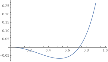
The score \(\varrho_2\) is particularly simple in this parametrization, as it depends only on \(\gamma\):
f = Simplify[Score2 //. P];
Plot[f, { γ, 0, 1 }]
sol = FindInstance[f == 0 && 0 < γ < 1, {γ}, Reals, 10];
{ Length[sol], sol[[1]], N[sol[[1]]]}
This produces the following plot of this function of \(\gamma\). FindInstance
is asked to provide ten roots of this function but only one is found which has approximate
value \(0.727662\).
We search for a non-negative tensor in the parametrized model whose \(\gamma\) is above the slightly lower threshold of \(0.727\), which is the only way to violate the Ingleton inequality in this parametrization. Out of all computations on this page, this takes the longest time:
sol = FindInstance[γ > 0.727 && And @@ Map[#[[2]] >= 0 &, P], {γ, ε, δ123, δ124}, Reals]
{}
This is a semialgebraic system, so \(\verb|Mathematica|\) will fall back to a symbolic algorithm such as cylindrical algebraic decomposition to decide the feasibility of the problem. It follows that there is no probability distribution in the part of the model parametrized by Matúš which has a positive non-Ingleton score.
Essential conditionality of the tenth inequality
The \(\verb|Mathematica|\) notebook containing the computations for Section 4 is available for download:
The combinatorial sampling inspired by counterexamples in the literature
is implemented in the function RandomDistribution[]. Distributions
from this sampling process are first filtered by a quick suitability test:
they must not already satisfy the CI assumptions for all \(\varepsilon\)
because then violation of Ingleton is impossible. But they must satisfy
them in the limit \(\varepsilon \to 0\).
vars = {p0000, p0001, p0010, p0011, p0100, p0101, p0110, p0111, p1000, p1001, p1010, p1011, p1100, p1101, p1110, p1111};
S1 = Simplify[-p0010*p1000-p0110*p1000+p0000*p1010+p0100*p1010-p0010*p1100-p0110*p1100+p0000*p1110+p0100*p1110 == 0 &&
  -p0011*p1001-p0111*p1001+p0001*p1011+p0101*p1011-p0011*p1101-p0111*p1101+p0001*p1111+p0101*p1111 == 0]
S2 = Simplify[-p0010*p0100+p0000*p0110+p0110*p1000-p0100*p1010-p0010*p1100-p1010*p1100+p0000*p1110+p1000*p1110 == 0 &&
  -p0011*p0101+p0001*p0111+p0111*p1001-p0101*p1011-p0011*p1101-p1011*p1101+p0001*p1111+p1001*p1111==0]

RandomGoodDistribution[] := Module[{p},
  While[True, p = RandomDistribution[];
    If[Not[And @@ {S1, S2} //. Catenate[{p, { \[Epsilon] -> 10^-10 }}]] &&
      And @@ {S1, S2} //. Catenate[{p, { \[Epsilon] -> 0 }}], Break[]]];
  p
]
As before we have functions to compute entropies and the following utility which extracts power series data from an expression:
SeriesOrder[F_, x_] := Module[{c = Series[Simplify[F], {x, 0, 4}]},
  If[SameQ[Head[c], SeriesData],
    { c[[3, 1]], c[[4]]/c[[6]] },
    If[c == 0, {0, Infinity}, {c, 0}]
  ]
];
Lim[F_, x_] := Limit[F, {x -> 0}, Direction -> "FromAbove"];
The criteria we use for a good distribution is: (a) Ingleton must vanish in the limit but (b) its highest-order power series coefficient must be negative for arbitrarily small \(\varepsilon\). This coefficient might still be a function of \(\varepsilon\) because \(\verb|Mathematica|\) recognizes that \(\varepsilon \log \varepsilon\) is not differentiable at \(0\) and thus excludes it from the power series expansion and then adds it back in. Hence we take the limit of the coefficient as \(\varepsilon \to 0\). Next, a distribution must either (c.1) give the Ingleton expression a strictly better convergence order than either of the two conditional mutual informations or at least, (c.2) if the orders are the same, the coefficient in Ingleton must tend to \(-\infty\) while the other two coefficients stay bounded.
 SelectFirst[Range[1000000], Module[{p, ing, acd, bcd},
   p = RandomGoodDistribution[];
   ing = SeriesOrder[Ingleton[p], \[Epsilon]];
   acd = SeriesOrder[iACD[p], \[Epsilon]];
   bcd = SeriesOrder[iBCD[p], \[Epsilon]];
   TimeConstrained[
     If[ing[[2]] > 0 && Lim[ing[[1]], \[Epsilon]] < 0 &&
       ((ing[[2]] < Min[acd[[2]], bcd[[2]]]) ||
        (ing[[2]] ==  Min[acd[[2]], bcd[[2]]] && Lim[ing[[1]], \[Epsilon]] == -Infinity &&
         Abs[Lim[acd[[1]], \[Epsilon]]] < Infinity && Abs[Lim[bcd[[1]], \[Epsilon]]] < Infinity)),
       Print[p, " is good"]; True],
     60, Print[p, " is unknown"]; False
   ]] &
];
Once a distribution is found at all, some parameters in RandomDistribution[]
can be fixed to focus the search on getting a particularly sparse counterexample.
At the end, we verify its properties symbolically again:
p = {p1111 -> 1/5, p1101 -> 1/5, p0110 -> 1/5, p1010 -> 1/5,
  p0010 -> 1/5 - \[Epsilon], p1100 -> \[Epsilon], p0100 -> 0,
  p0001 -> 0, p0111 -> 0, p0000 -> 0, p1011 -> 0, p0011 -> 0,
  p0101 -> 0, p1001 -> 0, p1000 -> 0, p1110 -> 0};
Series[Ingleton[p], {\[Epsilon], 0, 3}]
Simplify[iACD[p] == iBCD[p]]
Series[iACD[p], {\[Epsilon], 0, 3}]
System information
All computations were performed on the author’s laptop (a customary Thinkpad T580 with 16 GiB of RAM, although that much memory is never needed) using \(\verb|Perl|\) v5.30.1, \(\verb|CaDiCaL|\) v1.3.1, \(\verb|nbc_minisat_all|\) v1.0.2.b, \(\verb|Macaulay2|\) v1.16, \(\verb|4ti2|\) v1.6.9, \(\verb|Normaliz|\) v3.8.4 and \(\verb|Mathematica|\) v13.1.
Colophon
Project page created: 08/04/2022
Software used: Macaulay2 (v1.16), Mathematica (v11.3.)
Project contributors: Tobias Boege
Corresponding author of this page: Tobias Boege, tobias.boege@mis.mpg.de