S-EPGP demo

Imports, etc

## Imports
import torch
import matplotlib.pyplot as plt
import numpy as np
import pandas as pd
from pde import CartesianGrid, solve_laplace_equation

# Get cpu or gpu device for training.
device = "cuda" if torch.cuda.is_available() else "cpu"

torch.set_default_dtype(torch.float64)
torch.manual_seed(13);

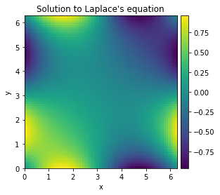
True solution

We compute a numerical solution to the Laplace equation in 2D: \(\partial_x^2 + \partial_y^2 = 0\).

grid = CartesianGrid([[0, 2 * np.pi]] * 2, 64)
bcs = [{"value": "sin(y)"}, {"value": "sin(x)"}]

res = solve_laplace_equation(grid, bcs)
res.plot();

We convert the py-pde types to PyTorch tensors

Ps = torch.tensor(grid.cell_coords)
u_true = torch.tensor(res.data)

Learning data will consist of randomly sampled points in the numerical solution

train_pts = 50
train_idx = torch.randperm(len(u_true.flatten()))[:train_pts]
X = Ps.flatten(0,1)[train_idx]
U = u_true.flatten()[train_idx]

Setting up a S-EPGP kernel

Running the command solvePDE in Macaulay2 reveals two varieties, namely the lines $ a = i b$ and \(a = - i b\), where \(a,b\) are spectral variables corresponding to \(x,y\) respecively. For both lines, there is only one Noetherian multiplier, namely 1. This means that the Ehrenpreis-Palamodov representation of solutions to Laplace’s equations are of the form

\[\int_{a = ib} e^{ax + by} \, d\mu_1(a,b) + \int_{a=-ib} e^{ax + by} \, d\mu_2(a,b)\]

By parametrizing the two lines, we can rewrite the integrals in a simpler form. We use the parametrizations

\[\begin{split}(a,b) = ((1+i)c, (1-i)c) \\ (a,b) = ((1-i)c, (1+i)c)\end{split}\]

The integrals then become

\[\int_{\mathbb C} e^{(1+i)cx + (1-i)cy} \, d\mu_1'(c) + \int_{\mathbb C} e^{(1-i)cx + (1+i)cy} \, d\mu_2'(c)\]

We approximate each measure with \(m\) Dirac delta measures. This translates to the S-EPGP kernel

\[k(x,y) = \Phi(x,y)^H \Sigma \Phi(x,y),\]

where \(\Phi(x,y)\) is the vector with entries

\[\begin{split}\Phi(x,y)_j = \begin{cases} e^{(1+i)c_jx + (1-i)c_jy}, & \text{if } j = 1,\dotsc,m \\ e^{(1-i)c_jx + (1+i)c_jy}, & \text{if } j = m+1, \dotsc, 2m \end{cases},\end{split}\]

and \(\Sigma\) is a \(2m \times 2m\) diagonal matrix with positive entries \(\sigma_j^2\).

Our goal will be to learn the \(c_j \in \mathbb C, \sigma_j^2 > 0\) that minimize the log-marginal likelihood.

Given an array c of length 2m and a s × 2 matrix X of points (x,y), the function Phi returns the 2m × s matrix with columns \(\Phi(x,y)\).

def Phi(c,X):
    c1, c2 = c.chunk(2)
    c1 = c1.unsqueeze(1) * torch.tensor([1+1.j,1-1.j])
    c2 = c2.unsqueeze(1) * torch.tensor([1-1.j,1+1.j])
    cc = torch.cat([c1,c2])
    return cc.inner(X).exp()

Objective function

Suppose we are trying to learn on \(s\) data points. Let \(X\) be the \(s \times 2\) matrix with input points \(x_k, y_k\), and \(U\) the \(s \times 1\) vector with output values \(u_k\). Let \(\Phi\) be the \(2m \times s\) matrix of features obtained by the function Phi above.

The negative log-marginal likelihood function is

\[\frac{1}{2\sigma_0^2}(U^TU - U^T\Phi^HA^{-1}\Phi U) + \frac{s - 2m}{2} \log \sigma_0^2 + \frac{1}{2} \log |A| + \frac{1}{2} \log |\Sigma| + \frac{n}{2} \log 2\pi,\]

where \(\sigma_0^2\) is a noise coefficient, and

\[A = \Phi \Phi^H + \sigma_0^2 \Sigma^{-1}\]

This can be computed efficiently using a Cholesky decomposition: \(A = LL^H\). Ignoring constants and exploiting the structure of \(\Sigma\), we get the objective function

\[\frac{1}{2\sigma^2}(\|U\|^2 - \|L^{-1}\Phi U\|^2) + \frac{s-2m}{2} \log \sigma_0^2 + \sum_{j=1}^{2m} \log L_{j,j} + \frac{1}{2} \sum_{j=1}^{2m} \log \sigma_j^2\]

The function below computes the Negative Log-Marginal Likelihood (NLML). Here we assume that Sigma is a length \(2m\) vector of values \(\log \sigma_j^2\), and sigma0 is \(\log \sigma_0^2\)

def NLML(X,U,c,Sigma,sigma0):
    phi = Phi(c,X)
    A = phi @ phi.H + torch.diag_embed((sigma0-Sigma).exp())
    L = torch.linalg.cholesky(A)
    alpha = torch.linalg.solve_triangular(L, phi @ U, upper=False)
    nlml = 1/(2*sigma0.exp()) * (U.norm().square() - alpha.norm().square())
    nlml += (phi.shape[1] - phi.shape[0])/2 * sigma0
    nlml += L.diag().real.log().sum()
    nlml += 1/2 * Sigma.sum()
    return nlml

Training

We now set up parameters, initial values, optimizers and the training routine. We will use \(m = 8\) Dirac delta measures for each integral.

m = 8
Sigma = torch.full((2*m,), -np.log(2*m)).requires_grad_()
sigma0 = torch.tensor(np.log(1e-5)).requires_grad_()
c = (1*torch.randn(2*m, dtype=torch.complex128)).requires_grad_()

U = U.to(torch.complex128).reshape(-1,1)
X = X.to(torch.complex128)

def train(opt, sched, epoch_max = 1000):
    for epoch in range(epoch_max):
        nlml = NLML(X,U,c,Sigma,sigma0)

        print(f'Epoch {epoch+1}/{epoch_max}\tNLML {nlml.detach():.3f}\tsigma0 {sigma0.exp():.3}\tc std {c.std():.3f}\tlr {sched.get_last_lr()[0]}', end='\r')

        opt.zero_grad()
        nlml.backward()
        opt.step()
        sched.step()

Here we use a simple Adam optimizer, with learning rate 0.1, and decaying by a factor of 10 every 1000 steps. We train for 3000 epochs.

opt = torch.optim.Adam([c,Sigma,sigma0], lr = 1e-2)
sched = torch.optim.lr_scheduler.StepLR(opt,3000,gamma=0.1)
train(opt,sched,3000)

Epoch 3000/3000 NLML -232.572   sigma0 7.4e-06  c std 0.695     lr 0.011

Prediction

Suppose we want to use our trained model to predict the value of the function at \(r\) points \((x,y)\), organized in the \(r \times 2\) matrix \(X_*\). We will do inference using the posterior mean, which is given by

\[\Phi_*^H A^{-1} \Phi U,\]

where \(\Phi_*\) is the \(2m \times r\) matrix, with columns \(\Phi(x,y)\) for each row in \(X_*\).

The following function computes the prediction, where the variable X_ corresponds to \(X_*\)

def predict(X_, X,U,c,Sigma,sigma0):
    with torch.no_grad():
        phi = Phi(c,X)
        A = phi @ phi.H + torch.diag_embed((sigma0-Sigma).exp())
        L = torch.linalg.cholesky(A)

        alpha = torch.linalg.solve_triangular(L, phi @ U, upper=False)
        alpha1 = torch.linalg.solve_triangular(L.H, alpha, upper=True)

        phi_ = Phi(c,X_)
        return (phi_.H @ alpha1).real

X_ = Ps.flatten(0,1).to(torch.complex128)
u_pred = predict(X_, X, U, c, Sigma, sigma0)

The root mean square error of our prediction is below

(u_pred.view_as(u_true) - u_true).square().mean().sqrt().item()

0.0003669123836532972

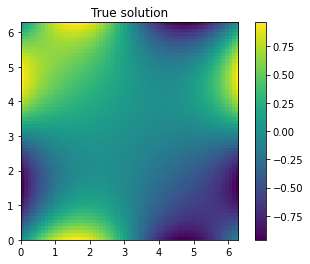
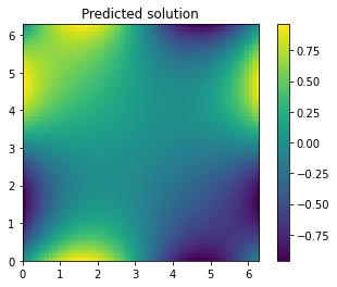
We can also visually compare the true solution with our prediction. The true solution is

ax = plt.imshow(u_true,extent=2*[0,2*np.pi])
plt.colorbar(ax)
plt.title("True solution");

ax = plt.imshow(u_pred.view_as(u_true),extent=2*[0,2*np.pi])
plt.colorbar(ax)
plt.title("Predicted solution");

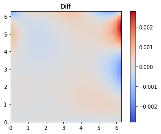
Finally, we plot the difference between the true and predicted solutions

diff = u_pred.view_as(u_true) - u_true
limit = max(diff.max(), -diff.min())
ax = plt.imshow(diff,extent=2*[0,2*np.pi], cmap='coolwarm', vmin = -limit, vmax = limit)
plt.colorbar(ax)
plt.title("Diff");