Principal A-Determinant of sparse arrangements

This notebook shows how to use the main features provided in the file PAD_Hyperplanes.jl.

If this is the first time you’re running Julia in a Jupyter notebook, run the following command line in the Julia terminal.

using Pkg; Pkg.add("IJulia")

For additional details about the optional input and the output of each function in the package we refer to the documentation written in the file PAD_Hyperplanes.jl before the implementation of each function.

We initiate the process by uploading the source file PAD_Hyperplanes.jl.

Note that in the upcoming step also automatically uploads Oscar. Instructions about the installation process of each package are provided at the page install_Oscar

include(string(pwd())*"/PAD_Hyperplanes.jl")

check_degree (generic function with 1 method)

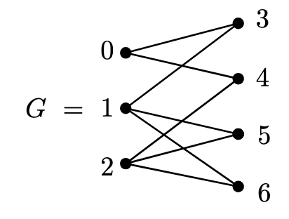
We test our code on the graph G = [V1,V2,E] from Example 3.5 in the article

G = [[0,1,2],[3,4,5,6],[[0,3],[0,4],[1,3],[1,5],[1,6],[2,4],[2,5],[2,6]]]

3-element Vector{Vector}:
 [0, 1, 2]
 [3, 4, 5, 6]
 [[0, 3], [0, 4], [1, 3], [1, 5], [1, 6], [2, 4], [2, 5], [2, 6]]

The function AfromG computes the matrix \(A_G\) with columns given by the vectors in the set in Equation (3.5)

A = AfromG(G)

7×8 Matrix{Int64}:
 1  1  0  0  0  0  0  0
 0  0  1  1  1  0  0  0
 0  0  0  0  0  1  1  1
 1  0  1  0  0  0  0  0
 0  1  0  0  0  1  0  0
 0  0  0  1  0  0  1  0
 0  0  0  0  1  0  0  1

The main function of our implementation uses Theorem 3.9 to compute the principal \(A\)-determinant of a complement of hyperplanes.

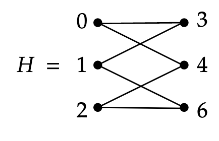
Applying the formula from Theorem 3.9 requires verifying certain conditions on specific subgraphs of the graph \(G\). The following code fragments illustrate the application of the functions that check these hypothesis to subgraphs.

I = [0,1,2]; J = [3,4,5];
H = subgraph(G,I,J)

3-element Vector{Vector}:
 [0, 1, 2]
 [3, 4, 5]
 [[0, 3], [0, 4], [1, 3], [1, 5], [2, 4], [2, 5]]

Using the function AfromGH we can compute the matrix \(A_{G/H}\) defined in Subsection 3.4. This matrix is the key ingredient to compute the multiplicities of the components of the principal \(A\)-determinant.

AGH = AfromGH(G,H)

1×2 Matrix{Int64}:
 1  1

The next function computes the subdiagram volume giving the multiplicity of the component of the principal \(A\)-determinant corresponding to the subgraph \(H\)

mH = subdiagram_volume(AGH)

1

The function my_is_connected checks if the subgraph induced by the sets \(I\subset V_1\) and \(J\subset V_2\) is connected

my_is_connected(G,I,J)

true

The function condition_star checks if the subgraph induced by the sets \(I\subset V_1\) and \(J\subset V_2\) verifies the part in condition \((*)\) defined in Subsection (3.3) concerning \(|V_1|>0\).

condition_star(G,I,J)

true

We can now compute the subgraphs of \(G\) contributing in the formula from Theorem 3.9.

The output below displays a list of pairs of type [[I,J],m], where \(I\subset V_1\) and \(J\subset V_2\) are such that the subgraph \(H=G_{I\cup J}\) of \(G\) leads to a non-defective face \(P_{H}\), and \(m\) is the corresponding multiplicity obtained via the subdiagram_volume function.

Here, we get the \(11\) factors from equation (3.12).

PAD = bipartite_A_determinant(G)

11-element Vector{Vector{Any}}:
 [[[0], [3]], 3]
 [[[0], [4]], 3]
 [[[1], [3]], 3]
 [[[1], [5]], 2]
 [[[1], [6]], 2]
 [[[2], [4]], 3]
 [[[2], [5]], 2]
 [[[2], [6]], 2]
 [[[1, 2], [5, 6]], 2]
 [[[0, 1, 2], [3, 4, 5]], 1]
 [[[0, 1, 2], [3, 4, 6]], 1]

The function check_degree performs a sanity check on the correctness of the result based on Proposition 2.4.

check_degree(G)

30

Example A: 3-site chain

G=[[0,1,2,3],[4,5,6,7,8,9],[[0,4],[0,5],[0,6],[0,7],[0,8],[0,9],[1,4],[1,5],[1,8],[2,4],[2,6],[2,8],[2,9],[3,4],[3,7],[3,9]]]

3-element Vector{Vector}:
 [0, 1, 2, 3]
 [4, 5, 6, 7, 8, 9]
 [[0, 4], [0, 5], [0, 6], [0, 7], [0, 8], [0, 9], [1, 4], [1, 5], [1, 8], [2, 4], [2, 6], [2, 8], [2, 9], [3, 4], [3, 7], [3, 9]]

PAD = bipartite_A_determinant(G)

58-element Vector{Vector{Any}}:
 [[[0], [4]], 1]
 [[[0], [5]], 11]
 [[[0], [6]], 9]
 [[[0], [7]], 11]
 [[[0], [8]], 3]
 [[[0], [9]], 3]
 [[[1], [4]], 8]
 [[[1], [5]], 11]
 [[[1], [8]], 8]
 [[[2], [4]], 4]
 ⋮
 [[[0, 1, 2, 3], [4, 5, 6, 7]], 1]
 [[[0, 1, 2, 3], [4, 5, 6, 9]], 1]
 [[[0, 1, 2, 3], [4, 5, 7, 8]], 1]
 [[[0, 1, 2, 3], [4, 5, 7, 9]], 1]
 [[[0, 1, 2, 3], [4, 5, 8, 9]], 1]
 [[[0, 1, 2, 3], [4, 6, 7, 8]], 1]
 [[[0, 1, 2, 3], [4, 6, 8, 9]], 1]
 [[[0, 1, 2, 3], [4, 7, 8, 9]], 1]
 [[[0, 1, 2, 3], [5, 7, 8, 9]], 1]

check_degree(G)

270