Euler Stratifications of Hypersurface Families

EulerStratifications.jl - a Julia package
We implemented the algorithms presented in our paper in the form of a Julia software package. The package can be found at here. To use the package execute the following commands in a terminal running Julia:
import Pkg
Pkg.add(url="https://github.com/maximilianwiesmann/EulerStratifications.jl")
using EulerStratifications
using Oscar
using HomotopyContinuation
In the following we explain how to reproduce the computational examples appearing in our paper.
Points on Smooth Curves (Example 3.5)
Example 3.5 computes the locus of lines in \((\mathbb{P}^2)^{\vee}\) which have at most \(\ell\) intersection points with the smooth plane curve \(X = V(x_0^3 - x_0x_2^2 - x_1^2x_2 + x_2^3) \subset \mathbb{P}^2\), for \(\ell \in \{1,2\}\).
R, (x,y,z) = graded_polynomial_ring(QQ, ["x","y","z"])  # create polynomial ring
f = x^3 - x*z^2 - y^2*z + z^3                           # polynomial defining X
d = Oscar.degree(Int, f)                                # degree of X
l = 1
get_stratum_smooth_curve(f, d-l)                        # compute stratum

l = 2
get_stratum_smooth_curve(f, d-l)                        # compute stratum
Note that the returned polynomials might not generate a radical ideal.
Projective Hypersurfaces (Examples 4.3 and 4.4)
In Example 4.3 we compute the Euler characteristic of the hypersurface complement \(\mathbb{P}^2 \setminus V(F)\), where \(F = x_0^3 + x_1^2x_2\) by computing the degrees of restrictions of the Gauss map.
@var x y z              # declare ModelKit variables
F = x^3 + y^2*z         # define polynomial
get_euler_char(F)       # compute Euler characteristic
In Example 4.4 we compute the polar discriminant of a generic ternary quadric
d, m = 2, 5
# create polynomial ring for parameters:
Rz, z = graded_polynomial_ring(QQ,["z$i" for i = 1:m+1])
# create polynomial ring for parameters and variables:
Rx, x = polynomial_ring(Rz,["x$i" for i = 1:d+1])
F = z[1]*x[1]^2 + z[2]*x[1]*x[2] + z[3]*x[1]*x[3] + z[4]*x[2]^2 + z[5]*x[2]*x[3] + z[6]*x[3]^2  # create polynomial
# possible parameter restriction (none in this case):
Iz = ideal([Rz(0)])
# compute polar discriminant:
get_polar_discriminant(F, Rz, Rx, Iz)
Very Affine Hypersurfaces (Example 5.9)
In Example 5.9 we present a complete Euler stratification for ternary quadrics in \((\mathbb{C}^*)^2\).
# define F, Rz, Rx and Iz as in previous example
euler_stratify(F, Rz, Rx, Iz; very_affine=true)      # compute Euler stratification in torus
Binary Octics in \(\mathbb{C}^*\) (Section 6.1)
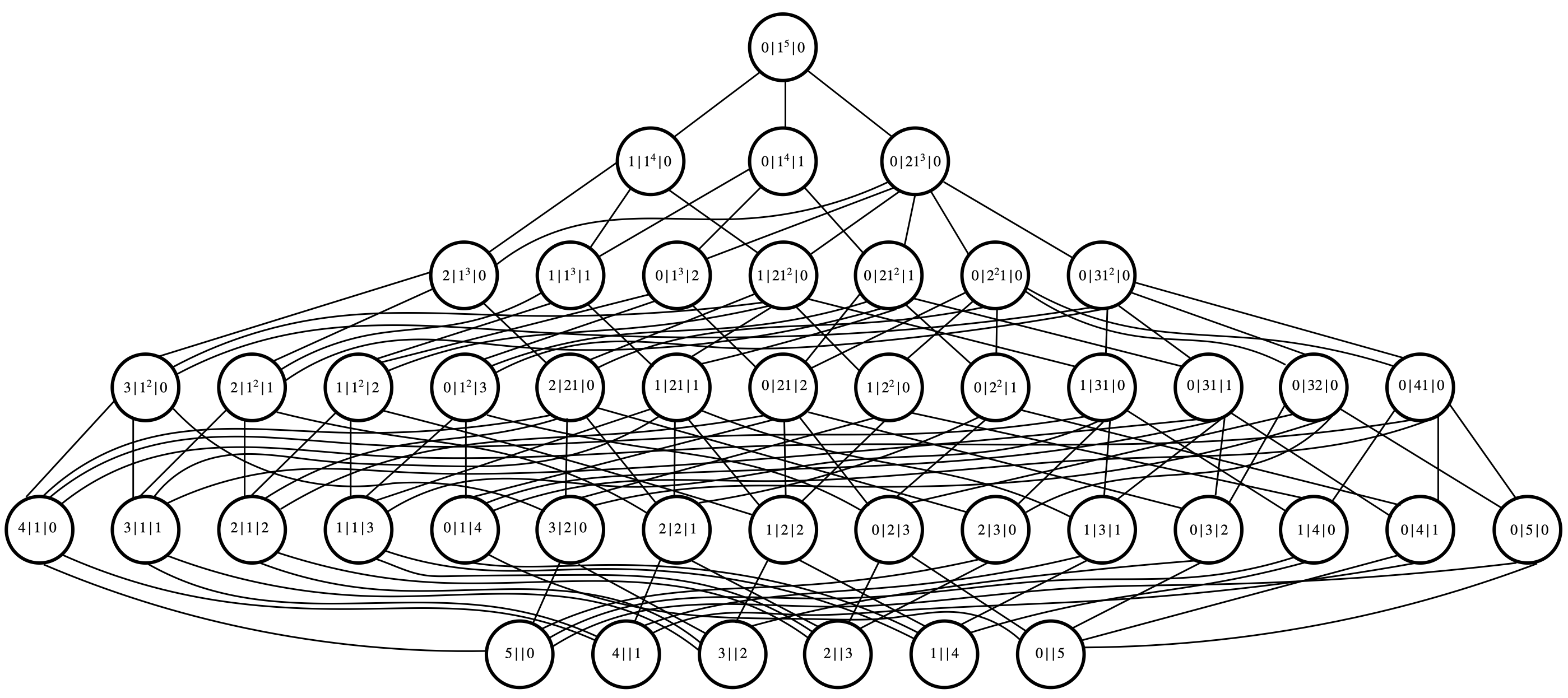
Here is a table where the ideals of the complete Euler stratification of a binary octic in \(\mathbb{C}^*\) can be downloaded (both as .txt-files displaying the generators and as .json-files which can be directly loaded into Oscar). The strata are labeled by decorated partitions. The figure below illustrates this for binary quintics:

Feynman Integrals (Section 6.3)

In Example 6.2 we compute the Euler stratification for the bubble graph (a).
d = 2
Rz, z = polynomial_ring(QQ, ["m_1";"m_2";"s"])
Rx, x = polynomial_ring(Rz, "x" => 1:d+1)
f = (x[3]-z[1]*x[1]-z[2]*x[2])*(x[1]+x[2]) + z[3]*x[1]*x[2]     # graph polynomial
Iz = ideal([Rz(0)])
euler_stratify(f, Rz, Rx, Iz; very_affine=true, randrange=-1000:1000)
In Example 6.3 we compute the Euler discriminant for the sunrise graph (b).
d = 3
Rz, z = polynomial_ring(QQ, ["m_1";"m_2";"m_3";"s"])
Rx, x = polynomial_ring(Rz, "x" => 1:d+1)
f = ((x[4]-sum([z[i]*x[i] for i = 1:3]))*(x[1]*x[2]+x[1]*x[3]+x[2]*x[3]) + z[4]*x[1]*x[2]*x[3])
Iz = ideal([Rz(0)])
get_euler_discriminant_veryaff(f, Rz, Rx, Iz)
In Example 6.4 we compute the Euler discriminant for the parachute graph (c).
d = 4
Rz, z = polynomial_ring(QQ, ["M_3"])
Rx, x = polynomial_ring(Rz, "x" => 1:d+1)
U = (x[1]+x[2])*(x[3]+x[4])+x[1]*x[2]
f = U*x[5] + z[1]*x[3]*x[4]*(x[1]+x[2]) - x[1]*x[2]*x[3] - (x[1] + 2*x[4])*U
Iz = ideal([Rz(0)])
get_euler_discriminant_veryaff(f, Rz, Rx, Iz; randrange=-1000:1000)
Toric Fano Varieties (Section 6.4)

In Example 6.5 we compute the complete Euler stratification for the GKZ families described by the five polytopes above.
A_3 = [0 1 1 2; 0 1 2 1]
A_4a = [1 0 1 2 1; 0 1 1 1 2]
A_4b = [1 0 1 2 1; 0 2 1 1 2]
A_4c = [1 0 1 2 1; 0 2 1 2 2]
A_5a = [1 0 1 2 1 0; 0 1 1 1 2 2]
stratify_GKZ(A_3)                       # Euler stratification for 3
Below are .txt-files containing generators for each of the ideals occurring in the stratifications of these five GKZ families.
Project page created: 22/07/2024.
Last updated: 16/04/2026.
Project contributors: Simon Telen, Maximilian Wiesmann.
Corresponding author of this page: Maximilian Wiesmann, wiesmann@pks.mpg.de.
Code written by: Simon Telen, Maximilian Wiesmann
Software used: Julia (Version 1.9.1), Oscar (Version 1.0.2), HomotopyContinuation.jl (Version 2.9.3).
System setup used: MacBook Pro with macOS Monterey 12.5, Processor Apple M1 Pro, Memory 16 GB LPDDR5.
License for code of this project page: MIT License (https://spdx.org/licenses/MIT.html).
License for all other content of this project page (text, images, …): CC BY 4.0 (https://creativecommons.org/licenses/by/4.0/).
Last updated 22/07/2024.