Fiber Convex Bodies
The Fiber Body of a Zonotope
Abstract: In this paper we study the fiber body, that is the extension of the notion of fiber polytopes for more general convex bodies. After giving an overview of the properties of the fiber body, we focus on three particular classes of convex bodies. First we describe the strict convexity of the fiber body of the so called puffed polytopes. Then we provide an explicit equation for the support function of the fiber body of some smooth convex bodies. Finally we give a formula that allows to compute the fiber body of a zonoid with a particular focus on the so called discotopes. Throughout the paper we illustrate our results with detailed examples.
This repository includes the code to compute the fiber body of a zonotope in \(\mathbb{R}^N\) with respect to its projection onto the first \(n\) coordinates. This is based on Corollary 5.10 in the paper.
We offer implementations written in \(\verb|OSCAR|\) and \(\verb|SageMath|\).
OSCAR
We load the following packages.
using Oscar
using IterTools
using LinearAlgebra
Given a list \(L = \{z_1,\ldots ,z_s \}\) of points in \(\mathbb{R}^N\), we can associate to it a zonotope, namely
where \([-z_i, z_i]\) is the segment between \(-z_i\) and \(z_i\). We can do this using the following function.
function zonotope(L)
    """
    Input:  list L
    Output: zonotope associated to L
    """
    sum(convex_hull([-ℓ; ℓ]) for ℓ in L)
end
The fiber body of the zonotope \(Z\) with respect to the projection \(\pi : \mathbb{R}^N\to \mathbb{R}^n\) onto the first \(n\) coordinates is the Minkowski sum
where \(F_\pi : (\mathbb{R}^n \times \mathbb{R}^{N-n})^{n+1}\to \mathbb{R}^{N-n}\) is defined by
The function fiber_zonotope takes as input the list \(L\) associated to the zonotope \(Z\) and returns as output the list of all \(F_\pi(z_{i_1},\ldots, z_{i_{n+1}})\).
function fiber_zonotope(L,n)
    """
    Input:  list L, associated to a zonotope Z
            integer n
    Output: list F_π, whose associated zonotope is the fiber zonotope of Z
            with respect to the projection onto the first n coordinates
    """
    N = length(L[1])
    s = length(L)
    X = [ℓ[1:n] for ℓ in L]
    Y = [ℓ[n+1:N] for ℓ in L]
    F_π = []
    for I in subsets(1:s,n+1)
        f = []
        for j in 1:n+1    # we compute now the summands of F_π
            II = copy(I)
            M = X[deleteat!(II,j)]
            MM = hcat(M...)
            dd = det(MM)
            g = 1/factorial(n+1)*(-1)^(n+1-j)*dd*hcat(Y[I[j]]...)
            push!(f,g)
        end
        F = factorial(n+1)*sum(f)    # this is F_π for the set of indices I
        append!(F_π, [F])
    end
    return F_π
end
Applying then zonotope to the list \(\verb|F_π|\) we obtain the fiber zonotope of \(Z\).
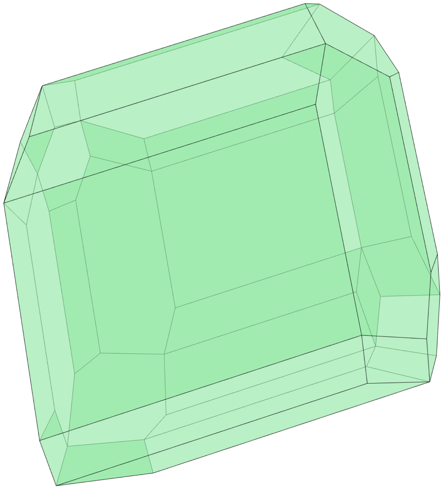
The image at the top of the page shows the polytope \(\verb|zonotope(fiber_zonotope(L))|\) for the list \(\verb|L = [[1 2 -3 1],[1 0 -1 0],[0 2 2 -1],[3 -2 1 2],[0 0 0 1],[1 1 1 1]]|\).
To download the Jupyter notebook that is displayed on the page, together with few examples, please click here.
SageMath
The Jupyter notebook fiber_zonotope_sagemath.ipynb contains the same functions described above for \(\verb|SageMath|\).