Hyperplane Arrangements in the Grassmannian
Numerically compute the Euler characteristic of Schubert hyperplane arrangements in Gr(k,n)
In Example 4.3 and Example 4.4, we use ML.jl to numerically compute the Euler characteristic of Schubert hyperplane arrangements in \(\text{Gr}(2,4),\text{Gr}(2,5)\).
It contains three parts.
NumCrit(d,k,n) (the main function): It counts the number of critical points of \(L=\sum_{i=1}^{d} c_i \log(\text{det}(M_i))\) with \(c_i\) random real numbers and \(M_i\) is the matrix obtained by stacking \((I,x)\) with a random real \((n-k,n)\) matrix
Examples
Polynomial interpolation of the points obtained by NumCrit(d,k,n) to compute the Euler characteristic
Sign patterns in \(\text{Gr}(k,n)\) without d hyperplanes
We provide code in SignPatterns.jl for randomly sampled points in \(\text{Gr}(k,n)\) without d hyperplanes and compute the sign patterns of the minors of the points.
Sign pattern, Euler characteristic and regions for \(\text{Gr}_\mathbb{R}(k,n)\) without d hyperplanes
Our computation is based on Algorithm 1 of arXiv:2405.18578 by Joseph Cummings, Jonathan D. Hauenstein, Hoon Hong and Clifford D. Smyth. A Julia package HypersurfaceRegions implementation is provided by Paul Breiding, Bernd Sturmfels and Kexin Wang, see arXiv:2409.09622 for more details.
Example 5.1
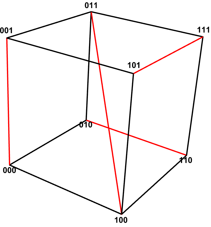
In Example 5.1, we study the complement of four Schubert Hyperplanes in \(\text{Gr}(2,4)\) corresponding to four \(2\times 4\) matrices:
They correspond to lines in \(\mathbb{P}^3\) that intersect the four lines connecting pairs of vertices in a (2,2,2,2) partition of 8 vertices in a unit cube.
We compute the regions in the affine chart \(\mathbb{R}^4\cong\text{Gr}_\mathbb{R}(2,4)-\{p_{12}=0\}\) with variables \(a, b, c, d\).
# define function that returns the equations for Schubert hyperplanes
function schubert_hyperplane(M)
    f=0
    set_size_2=[[3,4],[2,4],[1,4],[2,3],[1,3],[1,2]]
    poly_list=[1,-x21,-x11,x22,x12,x11*x22-x12*x21]
    for i in 1:6
        f+=poly_list[i]*det(M[:,set_size_2[i]])
    end
    return f
end
# input the matrices
M_2=[0 1 0 1; 1 1 0 1]
M_3=[1 0 1 1; 1 1 1 1]
M_4=[0 1 1 1; 1 0 0 1]

# define the system of equations for the Schubert hyperplanes
@var x11 x12 x21 x22
f_list=[]
M=[M_2,M_3,M_4]
for j in 1:3
    push!(f_list,schubert_hyperplane(M[j]))
end

# use HypersurfaceRegions.jl to compute the regions
import Pkg
Pkg.add("HypersurfaceRegions")
using HypersurfaceRegions
R=affine_region(f_list)
The output is as follows. There are eight sign patterns appeared and each of them has one region. For each region, we report its euler characteristic \(\chi\). We also report the tuple \(\mu\) consisting of the numbers of real critical points with certain index. For example, \(\mu = [1, 1, 0, 0, 0]\) means that there is one real critical point with index 0 and one real critical point with index 1.
RegionsResult with 8 regions:
=============================
44 complex critical points
26 real critical points
╭──────────────┬──────────────────────────────╮
│ sign pattern │ regions                      │
├──────────────┼──────────────────────────────┤
│ + - -        │ number = 1                   │
│              │  χ = 0,  μ = [1, 1, 0, 0, 0] │
│ - - +        │ number = 1                   │
│              │  χ = 0,  μ = [1, 1, 0, 0, 0] │
│ + + -        │ number = 1                   │
│              │  χ = 0,  μ = [2, 2, 0, 0, 0] │
│ - + +        │ number = 1                   │
│              │  χ = 0,  μ = [1, 1, 0, 0, 0] │
│ - - -        │ number = 1                   │
│              │  χ = 0,  μ = [2, 2, 0, 0, 0] │
│ - + -        │ number = 1                   │
│              │  χ = 0,  μ = [2, 2, 0, 0, 0] │
│ + - +        │ number = 1                   │
│              │  χ = -2, μ = [2, 4, 0, 0, 0] │
│ + + +        │ number = 1                   │
│              │  χ = 0,  μ = [1, 1, 0, 0, 0] │
╰──────────────┴──────────────────────────────╯
Example 5.2
Here is the code for the first example in Example 5.2
f_list=[x22,x11,x11*x22-x12*x21]

# use HypersurfaceRegions.jl to compute the regions
using HypersurfaceRegions
R=affine_regions(f_list)
The output is as follows. There are twelve sign patterns appeared and each of them contains one or two regions. For each region, we report its euler characteristic \(\chi\). We also report the tuple \(\mu\) consisting of the numbers of real critical points with certain index. Each region contains exactly one index 0 critical point, which implies that it is contractible.
RegionsResult with 12 regions:
==============================
20 complex critical points
12 real critical points

╭──────────────┬──────────────────────────────╮
│ sign pattern │ components                   │
├──────────────┼──────────────────────────────┤
│ - - +        │ number = 2                   │
│              │  χ = 1,  μ = [1, 0, 0, 0, 0] │
│              │  χ = 1,  μ = [1, 0, 0, 0, 0] │
│ + - -        │ number = 2                   │
│              │  χ = 1,  μ = [1, 0, 0, 0, 0] │
│              │  χ = 1,  μ = [1, 0, 0, 0, 0] │
│ - + +        │ number = 1                   │
│              │  χ = 1,  μ = [1, 0, 0, 0, 0] │
│ + + -        │ number = 1                   │
│              │  χ = 1,  μ = [1, 0, 0, 0, 0] │
│ - - -        │ number = 1                   │
│              │  χ = 1,  μ = [1, 0, 0, 0, 0] │
│ - + -        │ number = 2                   │
│              │  χ = 1,  μ = [1, 0, 0, 0, 0] │
│              │  χ = 1,  μ = [1, 0, 0, 0, 0] │
│ + - +        │ number = 1                   │
│              │  χ = 1,  μ = [1, 0, 0, 0, 0] │
│ + + +        │ number = 2                   │
│              │  χ = 1,  μ = [1, 0, 0, 0, 0] │
│              │  χ = 1,  μ = [1, 0, 0, 0, 0] │
╰──────────────┴──────────────────────────────╯
Here is the code for the second example in Example 5.2
# input matrices
M_2=[4 6 -10 2; 6 4 -5 -14]
M_3=[1 4 7 14; 26 0 -11 1]
M_4=[14 7 -4 -8; -6 7 2 7]

@var x11 x12 x21 x22

# define the system of equations for the Schubert hyperplanes
f_list=[]
M=[M_2,M_3,M_4]
for j in 1:3
    push!(f_list,schubert_hyperplane(M[j]))
end

# use Regions.jl to compute the regions
using HypersurfaceRegions
R=affine_regions(f_list)
RegionsResult with 9 regions:
=============================
44 complex critical points
28 real critical points

╭──────────────┬──────────────────────────────╮
│ sign pattern │ components                   │
├──────────────┼──────────────────────────────┤
│ - - +        │ number = 1                   │
│              │  χ = 0,  μ = [2, 2, 0, 0, 0] │
│ + - -        │ number = 1                   │
│              │  χ = 0,  μ = [1, 1, 0, 0, 0] │
│ - + +        │ number = 1                   │
│              │  χ = 0,  μ = [2, 2, 0, 0, 0] │
│ + + -        │ number = 1                   │
│              │  χ = -2, μ = [2, 4, 0, 0, 0] │
│ - - -        │ number = 2                   │
│              │  χ = 1,  μ = [1, 0, 0, 0, 0] │
│              │  χ = 1,  μ = [1, 0, 0, 0, 0] │
│ - + -        │ number = 1                   │
│              │  χ = 0,  μ = [2, 2, 0, 0, 0] │
│ + - +        │ number = 1                   │
│              │  χ = 0,  μ = [2, 2, 0, 0, 0] │
│ + + +        │ number = 1                   │
│              │  χ = 0,  μ = [1, 1, 0, 0, 0] │
╰──────────────┴──────────────────────────────╯
Example 5.3
We compute the number of regions in \(\text{Gr}_\mathbb{R}(2,4)\) for sampling \(n=4,5,6\) random Schubert hyperplanes in 100 trials. We always fix one Schubert hyperplane to be \(p_{12}=0\) and we sample the rest of them by sampling \(2\times 4\) matrices with standard Gaussian entries.
The data and code for this experiment can be downloaded via:
Project page created: 26/08/2024.
Project contributors: Elia Mazzucchelli, Dmitrii Pavlov, Kexin Wang
Corresponding author of this page: Kexin Wang, kexin_wang@g.harvard.edu.
Software used: Julia (Version 1.9.3), HomotopyContinuation.jl (Version 2.9.2), DifferentialEquations.jl (Version v7.11.0).
System setup used: MacBook Pro with macOS 13.5.2, Chip M2, Memory 16GB.
License for code of this project page: MIT License (https://spdx.org/licenses/MIT.html).
License for all other content of this project page (text, images, …): CC BY 4.0 (https://creativecommons.org/licenses/by/4.0/).
Last updated 26/08/2024.