Generic Identifiability vs. Non-Identifiability
We present Mathematica and Macaulay2 sessions reproducing the results given in Section 7, Table 1.
The Mathematica code that generates all non-simple graphs with a certain number of nodes and tests for generic identifiability
using the result in Lemma 3.3 (ii) is given in NonSimpleGenericID. The Macaulay2 code that
verifies non-identifiability of the graphs that seem to be not generically identifiable according to
the numerical test with Mathematica is given in
NonIdentifiability and
requires downloading LyapunovModel.
nodes |
total non-simple |
non-identifiable |
non-identifiable satisfying (7.1) |
|---|---|---|---|
3 |
2 |
0 |
0 |
4 |
80 |
3 |
2 |
5 |
4862 |
68 |
37 |
Non-simple graphs (Section 7) are never globally identifiable as they contain the non-identifiable 2-cycle \(G=(\lbrace 1,2 \rbrace, \lbrace 1 \to 2, 2 \to 1 \rbrace)\), see Example 2.4. However, if the number of parameters does not exceed the dimension of the positive-definite cone, the graphs can be either generically identifiable or non-identifiable. Consider Definition 2.1 for the different notions of identifiability.
Recall the result in Lemma 3.3. (ii). A graph \(G=(V,E)\) with \(V=[p]\) is generically identifiable if and only if there exists a matrix \(\Sigma \in \mathcal{M}_{G,C}\) such that \(A(\Sigma)_{\cdot, E}\) has full column rank \(|E|\).
The subsequent function takes the list of graphs as input and selects for every graph two matrices \(M_{1}^{*}\) and \(M_{2}^{*}\) that are supported over the graph and have prime numbers as entries. Then the function calculates the column rank \(A(\Sigma_{1}^{*})_{\cdot, E}\) and \(A(\Sigma_{2}^{*})_{\cdot, E}\). If at least one of the two column ranks are equal to \(|E|\), we conclude that the graph is generically identifiable. We omit displaying the code that gives the list of graphs with a certain number of nodes and simply present the function testing for generic identifiability.
--Function for testing for generic Identifiablity for a specific graph

genericidentifiability[graphlist0_,p0_]:=
Module[{graphlist=graphlist0,p=p0,M,M1,M2,S1,S2,L1,L2,A1,A2,L,M1t,M2t,graphc,index,zeroentries,nonzeroentries,nonzeroentriesl,i,j,k,A1l,M1l},


index=List[];
A1l=List[];
M1l=List[];
nonzeroentriesl=List[];
M1=ArrayReshape[RandomPrime[100,p^2],{p,p}];
M2=ArrayReshape[RandomPrime[100,p^2],{p,p}];

L=ConstantArray[0,{p,p}];
For[i=1,i<=p,i++,
        For[j=1,j<=p,j++,
                If[i != j,
                        L[[i,j]]={i,j}
                ]
        ]
];
L=DeleteCases[Flatten[L,1],0];

For[i=1,i<=Length[graphlist],i++,
        M1t=M1;
        M2t=M2;
        graphc=Complement[L,graphlist[[i]]];
        For[j=1,j<=Length[graphc],j++,
                M1t [[graphc[[j]][[1]],graphc[[j]][[2]]]]=0;
                M2t [[graphc[[j]][[1]],graphc[[j]][[2]]]]=0;
        ];
        zeroentries=List[];
        For[k=1,k<=p,k++,
                For[j=1,j<=p,j++,
                        If[M1t[[j,k]]==0,
                                zeroentries=AppendTo[zeroentries,(k-1)*p+j]
                        ];
                ];
        ];
        nonzeroentries=Complement[Table[x,{x,1,p^2}],zeroentries];
        S1=LyapunovSolve[M1t,-2*IdentityMatrix[p]];
        S2=LyapunovSolve[M2t,-2*IdentityMatrix[p]];
        M=Array[Subscript[m,##]&,{p,p}];
        L1=M.S1+S1.Transpose[M]+IdentityMatrix[p];
        L2=M.S2+S2.Transpose[M]+IdentityMatrix[p];
        A1=D[Flatten[L1],{DeleteCases[Flatten[Transpose[M]],0],1}];
        A1=DeleteDuplicates[A1][[All,nonzeroentries]];

        A1l=AppendTo[A1l,A1];
        M1l=AppendTo[M1l,M1t];
        nonzeroentriesl=AppendTo[nonzeroentriesl,nonzeroentries];

        A2=D[Flatten[L2],{DeleteCases[Flatten[Transpose[M]],0],1}];
        A2=DeleteDuplicates[A2][[All,nonzeroentries]];
        If[MatrixRank[A1]==Dimensions[A1][[2]]||MatrixRank[A2]==Dimensions[A2][[2]],
                index=AppendTo[index,i];
        ];
        ];
Return[List[M1l,A1l,index,nonzeroentriesl]];
]
With this first screening of the list of graphs we obtain that most of the non-simple graphs are generically identifiable.
To fill the third column of Table 1, we need to verify that the graph that seem to be not generically identifiable are
indeed non-identifiable. The list of graphs for \(p=5\) can be download in Graphlist5.
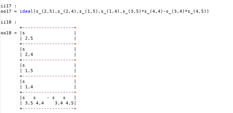
Before computing the column rank of \(A(\Sigma)_{\cdot, E}\), we identify the trek conditions (Corollary 7.3) that set
the entry \(\Sigma_{ij}=0\) whenever there is no trek from \(i\) to \(j\). As an example consider the graph below.
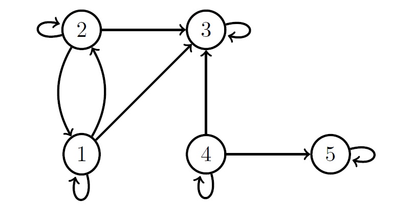
There are no treks between the pair of nodes (1,4),(1,5),(2,4) and (2,5).
-- STUDY OF NON-IDENTIFIABILITY OF NON-SIMPLE GRAPHS WITH 5 NODES
-- via A(Sigma) + trek conditions
-- via kernel of A(Sigma), which do not require trek conditions

restart
loadPackage "LyapunovModel";

-- load graphlist of graphs that seem to be non-identifiable

load "graphlist.txt";
L=value get "graphlist.txt";

--Computing trek conditions for a graph in the list

i=0; --choose graph
G=digraph({1,2,3,4,5},L_i)
(R,M,S)=lyapunovData G;
T=time trekIdeal(R,G);
betti (trim T)
netList (trim T)_*
i, length L_i  --position in the list, number of edges

(R,M,S)=lyapunovData G;
AS=ASigmaGraph(G)
T=time trekIdeal(R,G);
i, length L_i, numrows AS, numcols AS, rank AS
betti (trim T)
toString (trim T)
netList (trim T)_*Here would be the Mathematica code.
Having incorporated the trek conditions, we compute the column rank of \(A(\Sigma)_{\cdot, E}\) and check if it is equal to \(|E|\).
-- COMPUTE RESTRICTED A(SIGMA) WITHOUT RECOMPUTING GAUSSIANRING

G=digraph({1,2,3,4,5},L_0)
A=ASigma(G);

count=0;
for k in L do (G=digraph({1,2,3,4,5},k);
aux=A_(pattern G);
print(count,length k, numrows aux, numcols aux, rank aux);
count=count+1;)

count=0;
trickyGraphs={};
for k in L do (G=digraph({1,2,3,4,5},k);
aux=A_(pattern G);
if (numcols aux==rank aux) then trickyGraphs=append(trickyGraphs,count);
count=count+1;)
Alternatively, we can execute the check using the restricted kernel as described in Lemma 5.4.
-- COMPUTE RESTRICTED KERNEL WITHOUT RECOMPUTING GAUSSIANRING

restart
loadPackage "LyapunovModel";


G=digraph({1,2,3,4,5},L_0)
--compute matrix A(\Sigma)
A=ASigma G
(R,M,S)=lyapunovData G
--compute kernel
kern=syz A;


count=0;
for k in L do (GG=digraph({1,2,3,4,5},k);
HG=kern^(kernelPattern GG);
print(count,length k, numcols HG, numrows HG, rank HG);
count=count+1;)

-- Print only those that require additional checking

count=0;
trickyGraphs={};
for k in L do (GG=digraph({1,2,3,4,5},k);
HG=kern^(kernelPattern GG);
if (numrows HG==rank HG) then trickyGraphs=append(trickyGraphs,count);
count=count+1;)

length trickyGraphs -- 0
These examples were computed using Macaulay2, version 1.17, on a Surface Pro (2017) with a 2,6 GHz Intel Core i5-7300U processor and 8 GB.