Median filter algorithm

Back to main page

As described in Thresholding scheme & level set method, our median filter algorithm is an extension of the MBO scheme to the level set setting. Specifically, we choose a discretization of our domain \(D\) (and given measure \(\mu\)) by a point process \(P_N\). Additionally, we choose a kernel. In practice, this will often be a (normalized) characteristic function of a neighborhood domain (stencil). For now, we will consider the ball. Next, given an initial datum \(g:D\to\mathbb{R}\), we get the evolution by iteratively taking the median in the local stencil aroung each point simultaneously.

Figure 7. Visualization of the algorithm.

A visualization of this for a single point is shown in Figure 7.

Algorithm 1: The median filter scheme

Data: \(g\in \text{BUC}(D;\mathbb{R})\)

Result: Evolution \(u^n_h\)

\(u^0_h(x):= g(x)\ \forall x\in P_N\);

\(n\gets 0\);

while \(\frac{nh}{c_A}<T\) do

\(u^{n+1}_h(x):= \text{med}_N(u^n_h;A_r(x))\ \forall x\in P\);

\(n\gets n+1\);

end

The pseudo code is also shown in Algorithm 1. Here, \(h\) is the time step size (related to \(r\) by the parabolic scaling \(h=r^2\)) and \(\text{med}_N(u^n_h;A_r(x))\) denotes the local median of \(u_h^n\) in the neighborhood \(A_r\). This neighborhood is usually the ball of size \(r\). As a reminder, the median is the value in the middle in the sense that there are an equal number of values above and below it.

Figure 8. A simplified example of the algorithm.

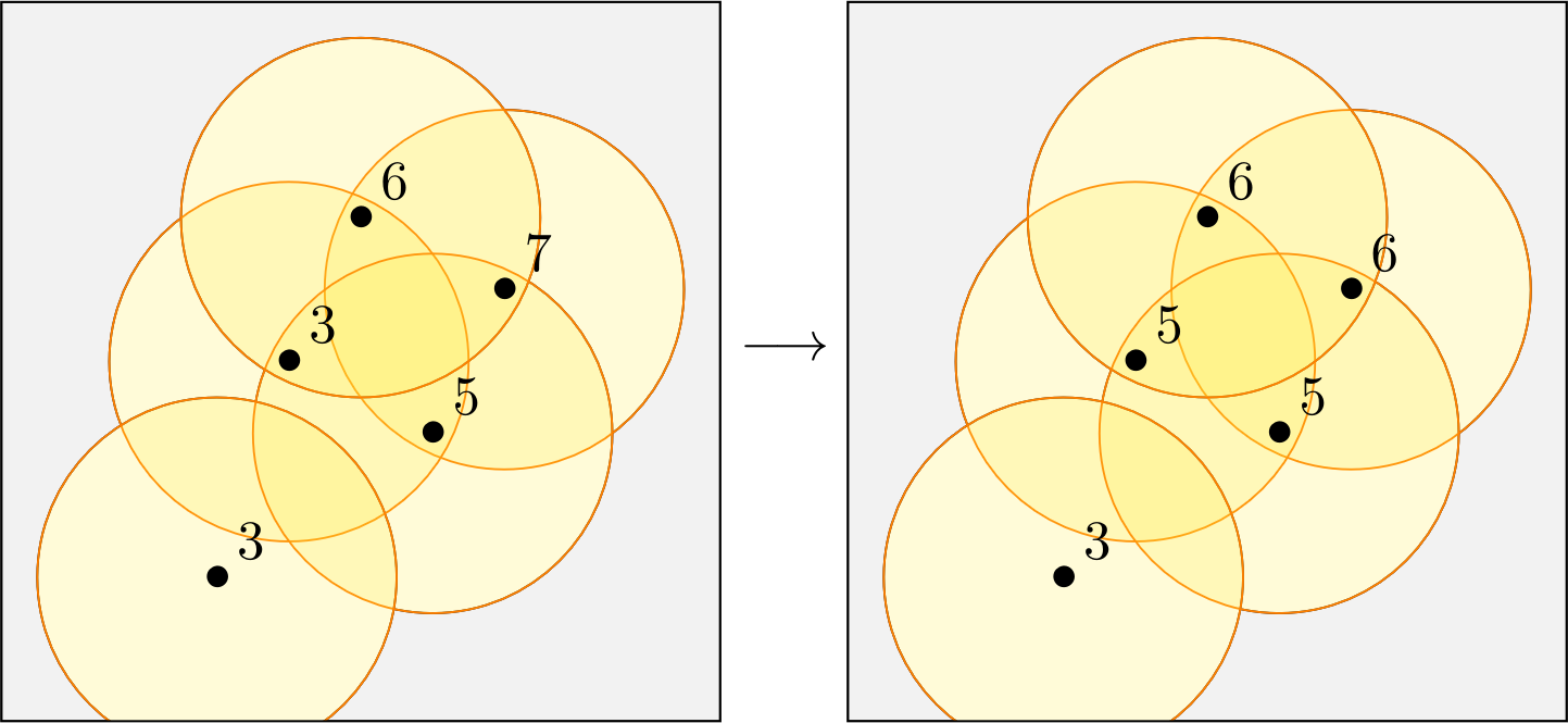
To visualize one step of the value update, one can look at Figure 8.

Intuitively this converges to MCF since the median is related to the level set Laplacian in the same way that the mean is related to the ordinary Laplacian.

An efficient implementation of our algorithm in rust can be found in MedianFilter.zip.

One could also use other kernels and domains for the algorithm. Partial results are also given for these cases.