Mean curvature flow
Back to main page
Mean curvature flow (MCF) is a flow on manifolds and can also be viewed
as a parabolic evolution equation on them. It is given by describing a
normal velocity \(V\) which depends on the curvature \(H\),
namely its describing equation is
\[V=-H.\]
This means that convex parts will shrink while concave parts grow, see
Figure 2 and Figure 3.
Figure 2. The evolution of a sphere \(\mathbb{S}^1\) in \(\mathbb{R}^2\).
In Figure 2, one can see the evolution of a one
dimensional sphere in \(\mathbb{R}^d\). Since the mean curvature of
a sphere \(\mathbb{S}^{d-1}_r\) is
\[H \equiv \frac{d-1}{r}\]
everywhere, the evolution is self-similar. Thus, the sphere/ball will
shrink with increasing velocity until it vanishes at time
\(t=\frac{r^2}{2(d-1)}\). An animation of this can be found in
Ball.mp4, see below.
Figure 3. The evolution of a curve with convex and concave parts in \(\mathbb{R}^2\).
Figure 3 shows the evolution of a curve in two
dimension that has convex and concave parts. By definition, the
convex parts will shrink while the concave parts will grow until they
become convex due to the global evolution. The whole evolution can be
found in
ConvConc.mp4, see below.
This already shows one of the most important properties of mean
curvature flow. It optimally dissipates the area, i.e. the surface area shrinks.
More precisely, MCF can be seen formally as a gradient flow on manifolds of the surface energy.
This gives rise to the specific name in two dimensions where MCF is also
called the curve shortening flow. In this case of \(d=2\), we have
more control and it holds that every smoothly embedded bounded curve
will becomes convex and shrinks to a round point in finite time. This
means that the curve will vanish in a point. Furthermore, the evolution will converge to a sphere in the Hausdorff distance if appropriately rescaled.
These theorems are due to Gage and Hamilton.
In higher dimensions more complex phenomena can occur. A special case
is the development of singularities in finite time. An example of this
is shown in Figure 4.
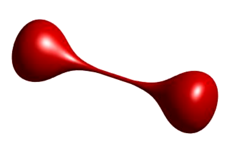
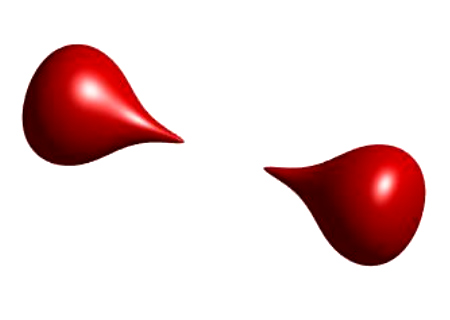
Figure 4. The evolution of the surface of a dumbbell in \(\mathbb{R}^3\).
In this figure, we observe the evolution of (the surface of) a
dumbbell. A video of this can be found in
Dumbbell.mp4, see below, which was created by
MBOScheme.m.
Here, the bar of the dumbbell undergoes a neck pinch and disappears before the rest. This can also be proven. Sketch–Singularity: For
this, we will need one of the most important tools available for general
evolutions associated with mean curvature flow, the comparison
principle. This principle states that two disjoint smooth manifolds
will evolve separately under MCF and won’t touch each other . For
this, a more useful formulation is obtained if we shift our
perspective from manifolds to sets. We will talk about the evolution of sets according to MCF when their boundaries evolve in this way. This change of perspective will also prove to be powerful in our
analysis and algorithms as we will see later.
Given this new perspective, the comparison principle (or maximum
principle) can be reformulated as the fact that if a set \(A\) is
contained in a set \(B\), their evolutions are ordered in the same way. Moreover, they will never meet. Using this, we can
observe that small balls vanish strictly faster than ones.
In addition, tori will vanish at least as fast as the smallest ball that contains them. So we can put a torus around the bar of the
dumbbell which is contained in a small ball while both ends of the
dumbbell contain large balls. Therefore, the neck must disappear before the ends.
Solution concepts: This already shows the need for general solution
concepts to talk about the evolution after the onset of singularities.
These singularities also occur only at a null set of times. A possible
unique extension is via viscosity solutions. We will mainly concentrate
on this concept but others are also viable. For these, see the
reference in the linked paper.
Applications
Mean curvature flow has a wide variety of applications.
Some of them are listed below. A typical application is the one of
crystal growth. A simulation of this is also shown in
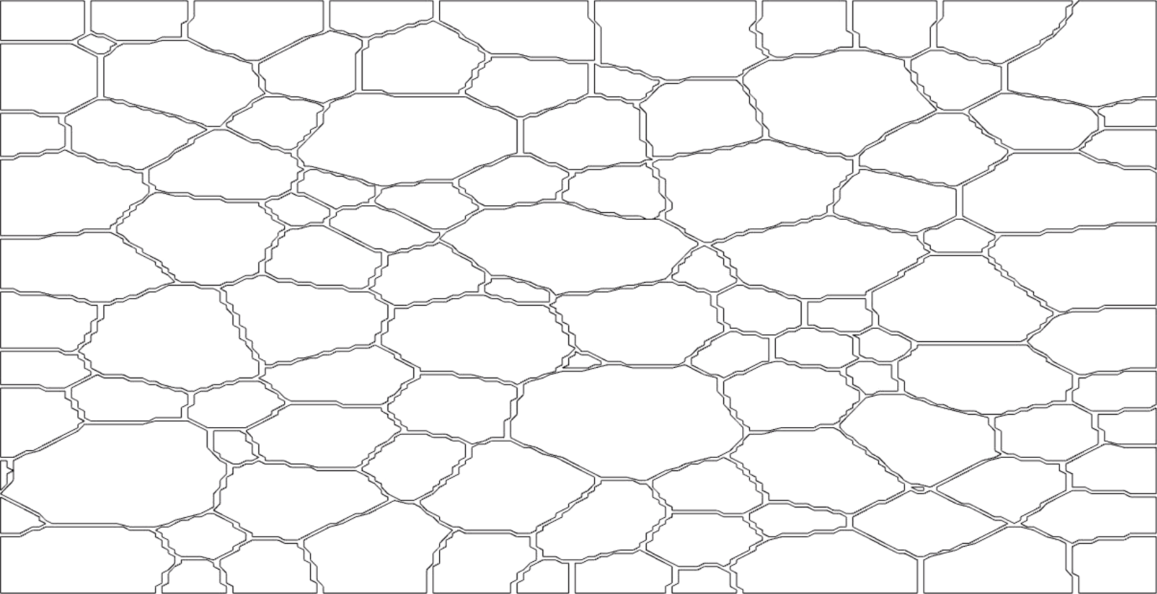
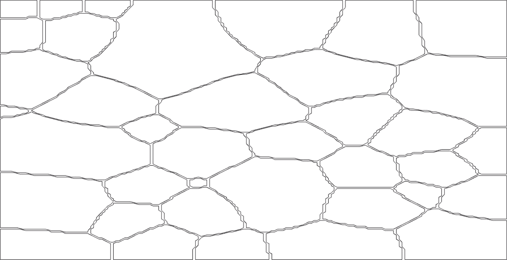
Figure 5.
In this figure, we see a simulation of a polycrystal (also called a
crystallite). Such crystals are formed when metals such as iron are cooled, for example, and can also be found in solar cells. In a nutrient
solution or under heating or similar conditions they undergo so-called
grain growth. This can be seen in the simulation and a video can be found
in Voronoi.avi.
Here, each grain (the cells) is a set evolving by mean curvature flow
and they are called phases. Thus, the whole evolution is an example of
multiphase MCF.
A related application is the analysis of material properties, since the grains influence e.g. how strong or malleable the material is. Other applications are more directly related to area minimization. These include the shape and analysis of soap films, as well as machine learning, image denoising, classification, and clustering algorithms.
Possible extensions of mean curvature flow include the evolution of
submanifolds on manifolds. Related to this, is the evolution on spaces
with densities or in domains with boundary. One could also analyze
anisotropic curvature flows.