Simulations

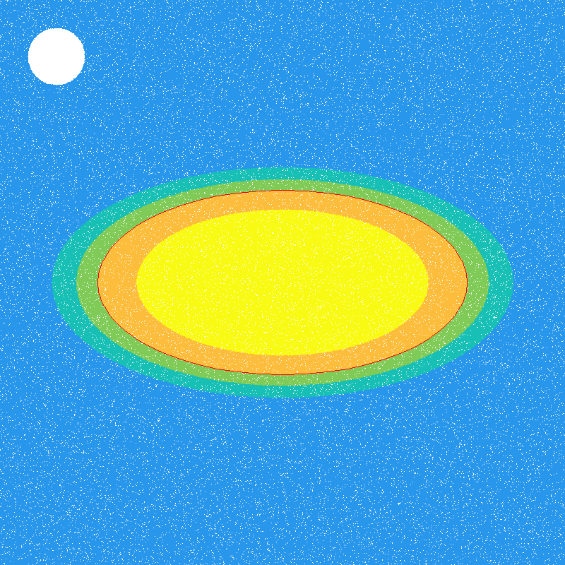
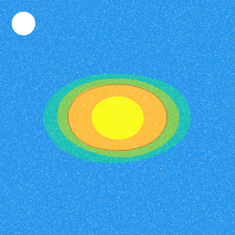
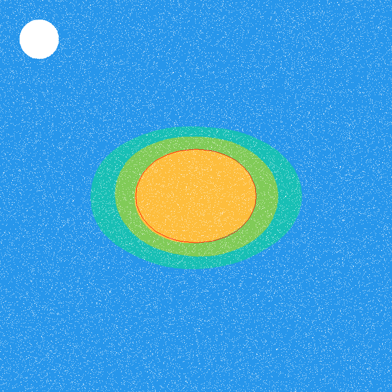
Figure 9. The evolution of a non-symmetric function.

Figure 9 shows the evolution of a function with ellipses as level sets. The white circle in the upper left corner shows which kernel was used in the simulation. Additionally, the red curve at the orange level set is a comparison to show the similarity to the (almost) exact evolution of a level set. This comparison was computed by a small step direct Euler method for a parameterization in tangential polar coordinates.

Classifier

Due to its nature as an area minimizing flow, the stationary sets are local minimizers, also called minimal surfaces. Thus, one can use the mean curvature flow algorithm to find classifiers.

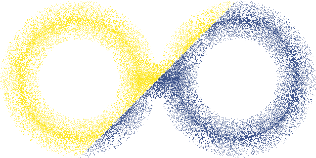
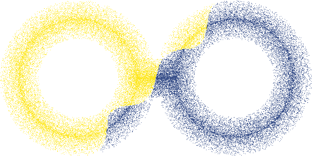
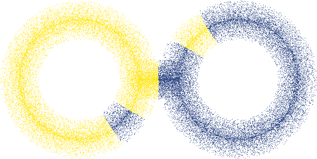
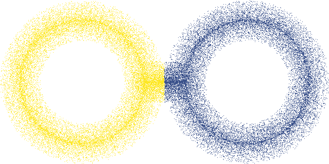
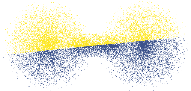
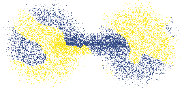
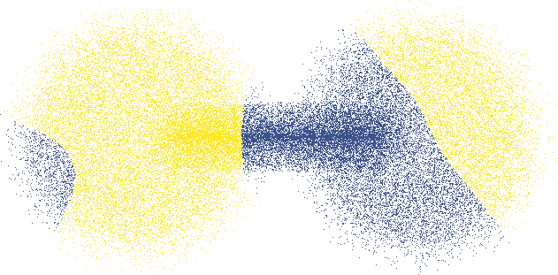
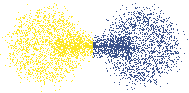
Some examples of this are shown above, where we assume that the objects shaped like dumbbells are manifolds representing our data. If they symbolize two classes of loosely connected sets, the optimal separation would be at the neck.

Young angle conditions

So far, all of our considerations neglected the boundary and the conditions we imposed there. This resulted in homogeneous Neumann conditions. That is, the level sets meet the boundary orthogonally and the gradient is perpendicular to the normal of the domain.

This can be generalized to Young angle conditions, i.e. we impose a fixed contact angle for all level sets. This can be achieved by changing the threshold depending on the position relative to the domain boundary. In terms of our level set function, this results in changing the median to a k-select. We don’t choose the value that lies in the middle but a different value depending on the desired percentage of values that should lie above our k-select value.

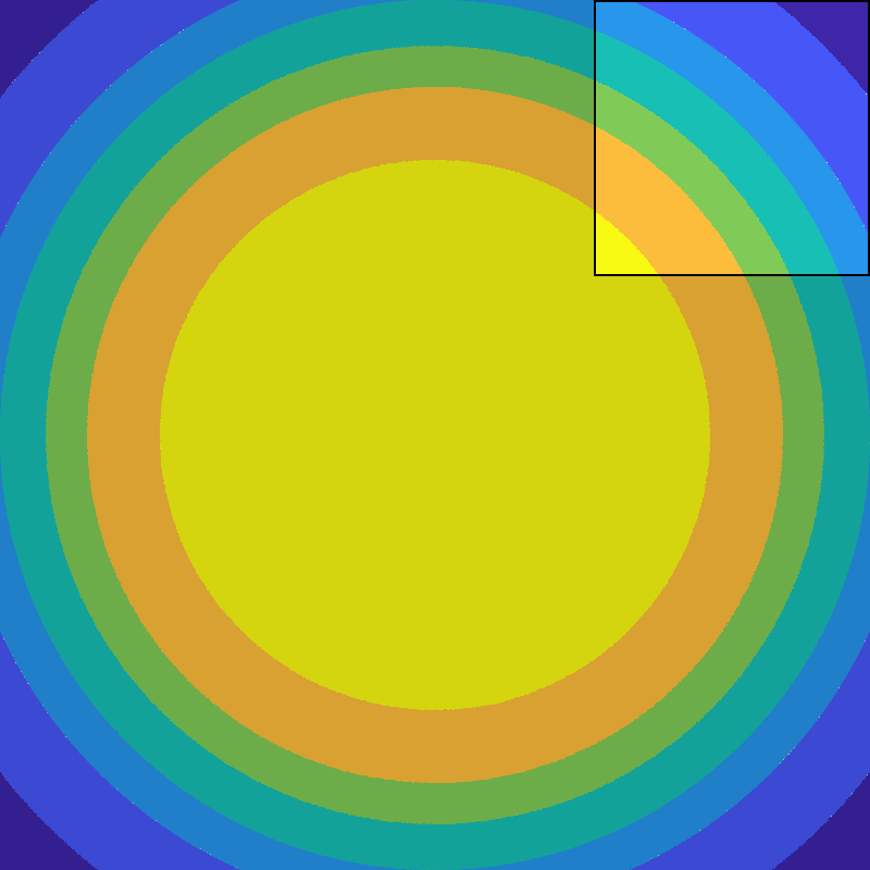
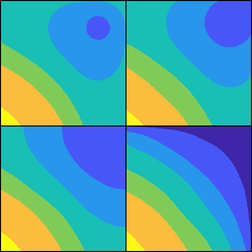
Figure 10. Evolution for different Young angle conditions.

Figure 11 shows the evolution of a quadratic radially symmetric function under different Neumann conditions. On the right is a zoom in of the upper right corner for four conditions is shown. The prescribed contact angles are \(0^\circ, 45^\circ, 90^\circ\) and \(180^\circ\).

The formulation of this scheme and the Young angle conditions results from an energy penalization of the common boundary with the domain.