Macaulay2 code and examples
For any staged tree, we can calculate its prime ideal and visually check whether this is generated by binomials as presented here.
In the first block of code below, we provide a number of functions which will enable us to input a tree parametrisation and, subsequently, study its algebraic properties. In particular, we give names to the rings we work over and set up notation for the tree structure in terms of inner vertices and leaves, creating the tree parametrisation as a ring map. We then use quotient operations to impose the conditions defining a statistical model, namely sum-to-one conditions and identifications across stages. This can be copied and pasted into any \(\verb|Macaulay2|\) compiler without requiring further packages.
-- create the probability (source) ring
probRing = method()
probRing(List) := (leaves) -> (
   R := QQ[for i in leaves list p_i];
   R
   )

-- create the list of indices of parameters
parameterIndices = method()
parameterIndices(List) := (leaves) -> (
   T := {};
   l := local l;
   i := local i;
   for l in leaves do(
        K := for  i in (0..#l-1) list (drop(l,-i));
        T =unique join(T,K));
   T
   )

-- create the parameter (target) ring
parameterRing = method()
parameterRing(List) := (leaves) -> (
   T := parameterIndices(leaves);
   S :=tensor(QQ[z],QQ[for i in T list s_i]);
   S
   )

-- collect sets of parameters that must sum to unity
sumto1 = method()
sumto1(List) := (leaves) -> (
   T := parameterIndices(leaves);
   psum1 := {};
   l := local l;
   t := local t;
   for t in T do(
        A := {};
        for l in T do(
           if t=!=l and drop(t,-1)==drop(l,-1) then  A=append(A,l));
           if A=!={} then  psum1=unique append(psum1,append(A,t)));
   psum1
   )

-- create the sum-to-one conditions
sumto1Eq = method()
sumto1Eq(List) := (leaves) -> (
   S := parameterRing(leaves);
   ps := sumto1(leaves);
   p := local p;
   i := local i;
   I := ideal(substitute(0,S));
for p in ps do(
   f := for i in p list s_i;
   I = I +ideal(substitute(1-(f//sum),S)));
   I
   )

-- create the stage conditions
stagedEq = method();
stagedEq(List) := (stages) -> (
   S := parameterRing(leaves);
   t := local t;
   i := local i;
   j := local j;
   k := local k;
   I := ideal(substitute(0,S));
   for t in stages do(
        for i in drop(t,1) do(
        for j in drop(t,1) do(
        for k from 1 to t_0 do(
        I = I+ideal(substitute(s_(append(i,k)),S)-substitute(s_(append(j,k)),S));
   ))));
   I
   )

-- target quotient ring taking in consideration sum-to-one and stage conditions
quotientRing= method()
quotientRing(List,List) := (leaves,stages) -> (
  S := parameterRing(leaves);
  I := ideal(substitute(mingens sumto1Eq(leaves),S));
  J := ideal(substitute(mingens stagedEq(stages),S));
quotS := S/(I+J);
quotS
)

-- create the staged tree's vanishing ideal
stagedIdeal = method()
stagedIdeal(List,List,Ring) := (leaves,stages,R) -> (
  S := parameterRing(leaves);
  quotS := quotientRing(leaves,stages);
  l := local l;
  imMap := {};
  for l in leaves do(
        use S;
        K := (for i in (0..#l-1) list s_(drop(l,-i)));
        imMap = append (imMap, substitute(product(K),quotS)));
  imMap = (substitute(z,quotS))*(toList imMap);
  psi = map(quotS,R,imMap);
  ker(psi)
)
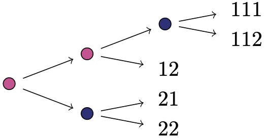
The above code can then be employed as illustrated below. Here, the input needed for the code above are leaves and stages. The labelling of vertices is as follows: label vertices inductively as lists of positive integers where the root is the empty list, and for a vertex with \(k\) children and label \(s\), its childrens are labeled by appending \(1\) through \(k\) to \(s\). Leaves obey this pattern, too. Each stage is given by the set of vertices in the same stage, together with the number of their outgoing edges. This number is put first. Stages is a set containing each stage. We illustrate this labelling in the picture below.
-- EXAMPLE 7.2 in the paper
-- input
leaves = {{1,1,1},{1,1,2},{1,2},{2,1},{2,2}}
stages = {{2,{},{1}},{2,{2},{1,1}}}
-- methods from above
R = probRing(leaves) --source ring where the ideal lives
I = stagedIdeal(leaves,stages,R) --the staged tree's vanishing ideal
S = QQ[p_1..p_(length(leaves))];
M = map(R,S,
    {p_{1,1,1}+p_{1,1,2},
    p_{1,1,2},
    p_{1,1,1}+p_{1,1,2}+2*p_{1,2},
    p_{1,1,1}+p_{1,1,2}+4*p_{2,1}+4*p_{2,2},
    p_{1,1,2}+4*p_{2,2}}
    )
-- output
Minv = inverse M
Iinv = trim Minv(I) --toric ideal obtained from linear change of coordinates
-- other notions
parameterIndices(leaves)
S = parameterRing(leaves)
psum1 = sumto1(leaves)
sumto1Eq(leaves)
stagedEq(stages)
quotientRing(leaves,stages)
Finally, for all trees in Figure 11 in our paper, we provide computations which find linear transformations revealing their respective toric structure. These can be downloaded here Figure11.m2 and carried out with the file Ideals_of_Staged_Trees.m2 in the same folder. The latter contains all the code and functions inside the first box on this page. On our system setup, the computation of these features for each tree took less than 0.4 seconds.