Mathematica discussion and examples

In general, it is difficult to balance the benefits of a wider search range for transformation matrices against the probability of finding transformations which have any equal entries at all (and can thus provide an isomorphism between between old variables \(p_1,\ldots,p_n\) and new \(q_1,\ldots,q_n\)). To see this, consider a stage represented by a matrix of dimension \(k\times l\). If we allow only transformations using integer entries with \(r,s\) choices of these for the transformation matrices multiplied from the left and right, respectively, then there are \(r^{k^2}\) candidate transformation matrices from the left, and equivalently for the right hand side and \(l\) and \(s\). Most of these matrices are invertible, as the set of invertible matrices over \(\mathbb{R}\) is dense in the set of all square matrices over \(\mathbb{R}\). Picking pairs of these candidate transformations grows exponentially in the number of entries allowed and has to be done for every stage in the model, subsequently counting whether the number of distinct entries of all of these equals the number \(n\) of atoms in the model. It is thus not surprising that some of the examples in our paper and in the list below cannot be decided: there is no evidence against them being toric but there could always be an adequate parametrisation which we have not yet been able to find.

Example 0: creating invertible matrices with integer entries

We can create a list of transformation matrices with the following simple command.

invertibleinteger[Range[-1,2],2,100]

This provides one hundred \(2\times 2\) matrices with integer entries in \(\{-1,0,1,2\}\) almost instantaneously.

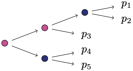
Example 1: a square-free and stratified balanced staged tree

Consider a staged tree representing a full independence model between a binary and a ternary random variable. This can be characterised using the equations \(p_1p_5=p_4p_2, (p_1+p_2)p_6=p_3(p_4+p_5)\). Its ideal of model invariants is known to be generated by binomials in the \(p\)-variables using the concept of path extensions from Duarte and Görgen (2018). We run the following piece of code to check our computations and verify this result.

lineartransform[{{{p1, p3}, {p2, p4}}, {{p1 + p2, p4 + p5}, {p3, p6}}},
                6, ConstantArray[{Range[-1, 1], Range[-1, 1]}, 2], 100000]

In a hundred thousand random trials this found about fifty transformations in new variables, resulting for instance in the reparametrisation \(q_1=-p_3-p_4, q_2=p_1+p_2, q_3=-p_3, q_4=p_1, q_5=-p_1-p_2-p_4-p_5, q_6=p_3+p_6\) which gives binomial generators of the staged tree’s prime ideal.

Example 2a: a non-squarefree, toric staged tree

The non-squarefree staged tree below fulfils the subtree-inclusion property and is hence toric.

We can look for a reparametrisation of the defining equations \(p_1p_4=p_3p_2, (p_1+p_2)p_5=(p_1+p_2+p_3+p_4)(p_3+p_4)\), \((p_1+p_2)p_6=(p_1+p_2+p_3+p_4+p_5)(p_3+p_4)\), and \((p_1+p_2+p_3+p_4)p_6=(p_1+p_2+p_3+p_4+p_5)p_5\) using the following command.

lineartransform[{{{p1, p3}, {p2, p4}},
                {{p1 + p2, p1 + p2 + p3 + p4, p1 + p2 + p3 + p4 + p5}, {p3 + p4, p5, p6}}},
                7, ConstantArray[{Range[-1, 1], Range[-1, 1]}, 2], 1000000]

This finds about 250 possible transformations, confirming that this staged tree represents a toric variety. Its prime ideal can, for instance, be generated by binomials in the variables \(q_1=p_1, q_2=p_1+p_3, q_3=p_1+p_2, q_4=p_1+p_2+p_3+p_4, q_5=p_5, q_6=-p_5+p_6,q_7=p_3+p_4\).

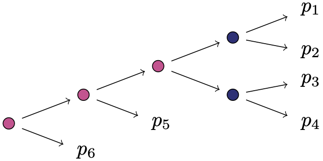
Example 2b: another non-squarefree, toric staged tree

The following staged tree is not square-free and does not fulfil the criteria we present in the paper to check whether it is toric.

We use our code to look for transformations in a certain range with weighted probabilities.

lineartransform[{{{p1, p4}, {p2, p5}}, {{p1 + p2, p1 + p2 + p3}, {p3, p4 + p5}}}, 5,
                {{{0.25, 0.75} -> {0, 1}, {0.25, 0.5, 0.25} -> {0, 1, 4}},
                {{0.25, 0.5, 0.25} -> {0, 1, 2}, {0.25, 0.25, 0.25, 0.25} -> Range[-1, 2]}},
                1000000]

This finds about two dozen possible reparametrisations, so the staged tree represents a toric variety. Its prime ideal can, for instance, be generated by binomials in the variables \(q_1=p_1, q_2=p_1+4p_4, q_3=p_1+p_2,p_1+p_2+4(p_4+p_5), q_4=p_1+p_2+2p_3, q_5=p_1+p_2+2p_3\), giving a characterisation of the model in terms of the equations \(q_1q_4 = q_2q_3\) and \(q_5^2 = q_3q_4\).

Example 3: a staged tree whose structure is currently not known

The following is a staged tree with a lot of symmetry which is not captured by any of the theoretical results in our paper.

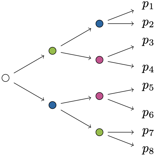
In order to decide whether it might have toric structure, we run the following code:

lineartransform[{{{p1, p5 + p6}, {p2, p7 + p8}}, {{p1 + p2, p3 + p4}, {p7, p8}}, {{p3, p5}, {p4, p6}}},
                8, ConstantArray[{Range[-1, 1], Range[-1, 1]}, 3], 1000000]

On repeated iterations, this did not yield any binomial generators for its ideal of model invariants. As of now, it is undecided whether this has toric structure.