Running example: the 4-claw tree
We present Macaulay2 sessions reproducing the running example of our paper (Examples 3.3, 3.6, 4.1, 4.11 and 6.5).
The full code can be found in Running example, and requires downloading MomentsVarieties.m2.
Let \(G\) be the DAG with edges \(1\rightarrow 2,\,1\rightarrow 3,\,1\rightarrow 4,\,1\rightarrow 5\). \(G\) gives rise to the linear structural equation model consisting of the joint distributions of all random vectors \(X= (X_1,X_2,X_3,X_4)\) such that
where the \(\varepsilon_i\) are mutually independent random variables with zero mean representing stochastic errors.
We consider the model \(\mathcal{M}^{\leq 3}(G)\) of covariance matrices and third-order tensors of the joint distributions of random vectors \(X\) defined as above.
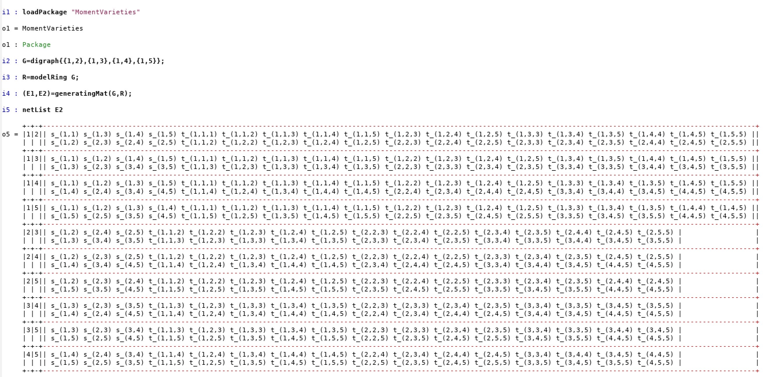
We first compute all trek-matrices (Definition 3.2) associated to this graph (see Example 3.3).
loadPackage "MomentVarieties"
G=digraph{{1,2},{1,3},{1,4},{1,5}}
R=modelRing G
(E1,E2)=generatingMat(G,R);

-- E2 lists all trek-matrices:
netList E2
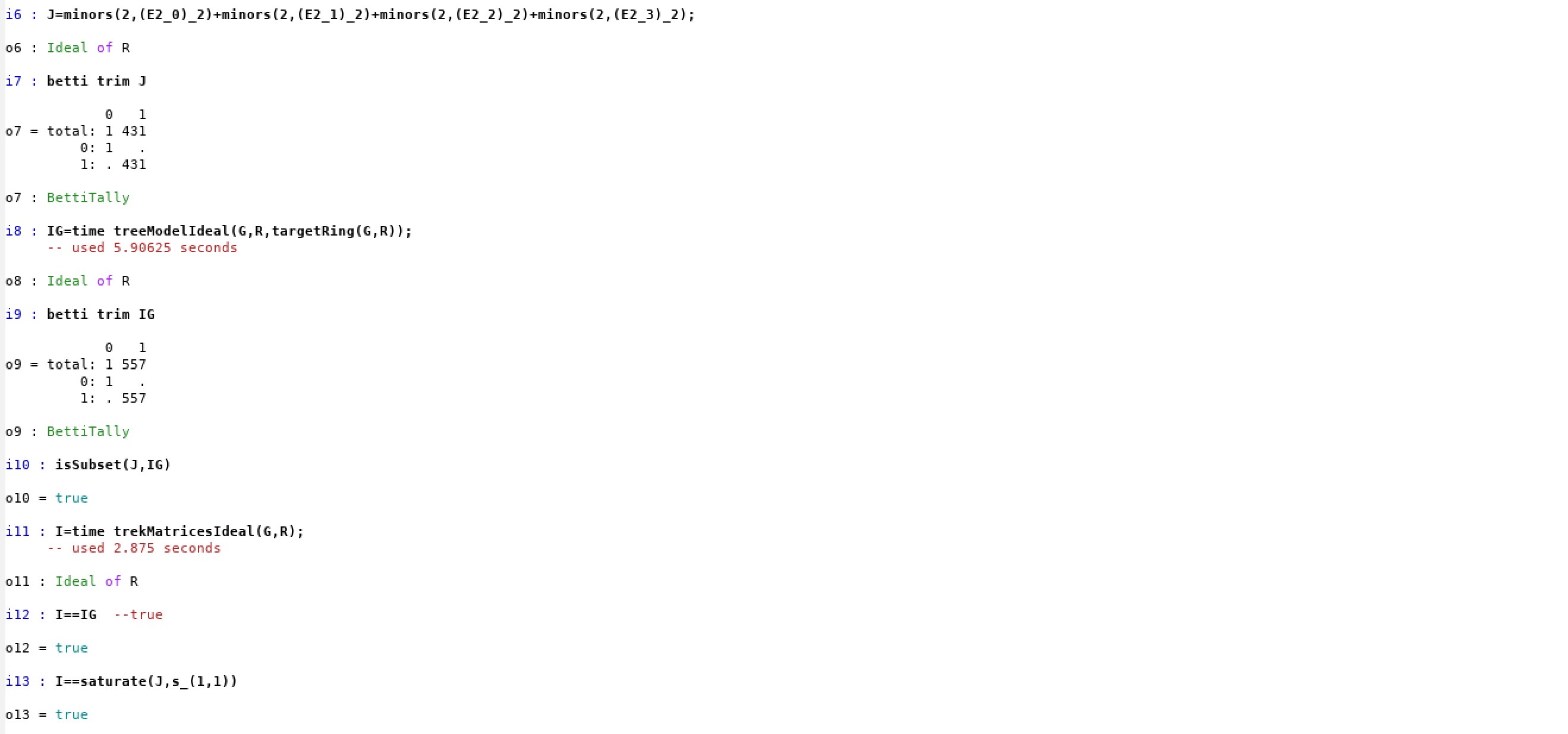
Next we compute the ideal \(J\) arising from trek-matrices corresponding to directed edges (see Example 3.6) and the vanishing ideal \(\mathcal{I}^{\leq 3}(G)\) of the model (see Example 4.1). It can be checked that \(J\) is contained but not equal to \(\mathcal{I^{\leq 3}}(G)\). We double-check that the ideal generated by all trek-matrices is indeed the vanishing ideal of the model. The relation between the two ideals is explained by saturation (see Example 4.11).
-- ideal of 2-minors of trek-matrices corresponding to directed edges:
J=minors(2,(E2_0)_2)+minors(2,(E2_1)_2)+minors(2,(E2_2)_2)+minors(2,(E2_3)_2);
betti trim J

--kernel of the monomial parametrization
IG=time treeModelIdeal(G,R,targetRing(G,R));
betti trim IG
isSubset(J,IG) --true

--ideal generated by all trek-matrices (and variables if needed)
I=time trekMatricesIdeal(G,R);
I==IG  --true

--relation between the vanishing ideal of the model and
--the ideal of 2-minors of trek-matrices corresponding to directed edges
I==saturate(J,s_(1,1))
Finally, we display the code that explores all possible degree reverse lexicographic term orders and shows that there exists no such order giving a squarefree initial ideal (see Example 6.5).
-- list of variables corresponding to each one of the seven categories:
L={{t_(2,2,2),t_(3,3,3),t_(4,4,4),t_(5,5,5)}, --t_iii
   {t_(1,1,1)},                               --t_111
   {t_(1,2,2),t_(1,3,3),t_(1,4,4),t_(1,5,5)}, --t_1ii
   {t_(1,1,3),t_(1,1,2),t_(1,1,4),t_(1,1,5)},  --t_11i
   {t_(2,3,3),t_(2,4,4),t_(2,5,5),t_(3,4,4),t_(3,5,5),t_(4,5,5),--t_ijj
    t_(2,2,3),t_(2,2,4),t_(2,2,5),t_(3,3,4),t_(3,3,5),t_(4,4,5)},
   {t_(1,3,5),t_(1,3,4),t_(1,4,5),t_(1,2,3),t_(1,2,5),t_(1,2,4)},--t_1jk
   {t_(2,3,4),t_(2,3,5),t_(2,4,5),t_(3,4,5)}} --t_ijk

netList L

-- quadratic binomials in the ideal that give restrictions on the orders
(t_(1,1,1)*t_(1,2,2)-t_(1,1,2)^2) % IG  --t_111*t_1jj-t_11j^2
-- t_111 > t_11i
-- t_1ii > t_11i
(t_(1,2,2)*t_(1,3,3)-t_(1,2,3)^2) % IG  --t_1ii*t_1jj-t_1ij^2
-- t_1ii > t_1ij
(t_(1,1,2)*t_(2,3,3)-t_(1,2,3)^2) % IG  --t_11i*t_ijj-t_1ij^2
-- t_11i > t_1ij
-- t_ijj > t_1ij
(t_(2,2,3)*t_(3,4,4)-t_(2,3,4)^2) % IG  --t_iij*t_jkk-t_ijk^2
-- t_iij > t_ijk

-- list of all orders satisfying:
-- t_111,t_1ii > t_11i > t_1ij
-- t_iij > t_1ij, t_ijk

V={{L_0,L_1,L_2,L_3,L_4,L_5,L_6},   --t_111>t_iii>t_1jj>t_11j>t_iij>t_1jk>t_ijk
   {L_0,L_1,L_2,L_3,L_4,L_6,L_5},
   {L_0,L_1,L_2,L_4,L_3,L_5,L_6},
   {L_0,L_1,L_2,L_4,L_3,L_6,L_5},
   {L_0,L_1,L_2,L_4,L_6,L_3,L_5},
   {L_0,L_1,L_4,L_2,L_3,L_5,L_6},
   {L_0,L_1,L_4,L_2,L_3,L_6,L_5},
   {L_0,L_1,L_4,L_2,L_6,L_3,L_5},
   {L_0,L_1,L_4,L_6,L_2,L_3,L_5},
   {L_0,L_4,L_1,L_2,L_3,L_5,L_6},
   {L_0,L_4,L_1,L_2,L_3,L_6,L_5},
   {L_0,L_4,L_1,L_2,L_6,L_3,L_5},
   {L_0,L_4,L_1,L_6,L_2,L_3,L_5},
   {L_0,L_4,L_6,L_1,L_2,L_3,L_5},
   {L_0,L_2,L_1,L_3,L_4,L_5,L_6},
   {L_0,L_2,L_1,L_3,L_4,L_6,L_5},
   {L_0,L_2,L_1,L_4,L_3,L_5,L_6},
   {L_0,L_2,L_1,L_4,L_3,L_6,L_5},
   {L_0,L_2,L_1,L_4,L_6,L_3,L_5},
   {L_0,L_2,L_4,L_1,L_3,L_5,L_6},
   {L_0,L_2,L_4,L_1,L_3,L_6,L_5},
   {L_0,L_2,L_4,L_1,L_6,L_3,L_5},
   {L_0,L_2,L_4,L_6,L_1,L_3,L_5},
   {L_0,L_4,L_2,L_1,L_3,L_5,L_6},
   {L_0,L_4,L_2,L_1,L_3,L_6,L_5},
   {L_0,L_4,L_2,L_1,L_6,L_3,L_5},
   {L_0,L_4,L_2,L_6,L_1,L_3,L_5},
   {L_0,L_4,L_6,L_2,L_1,L_3,L_5}};

#V

for v in V do {
S=QQ[flatten V_0];
IS=trim sub(IG,S);
JS=ideal leadTerm(1,IS);
print isSquareFree monomialIdeal JS;
print betti JS;
print (ideal gens gb IS)_306}
These examples were computed using Macaulay2, version 1.17, on a Surface Pro (2017) with a 2,6 GHz Intel Core i5-7300U processor and 8 GB.