Average degree of the essential variety
Abstract of the paper. The essential variety is an algebraic subvariety of dimension \(5\) in real projective space \(\mathbb R\mathrm P^{8}\) which encodes the relative pose of two calibrated pinhole cameras. The \(5\)-point algorithm in computer vision computes the real points in the intersection of the essential variety with a linear space of codimension \(5\). The degree of the essential variety is \(10\), so this intersection consists of \(10\) complex points in general.
We compute the expected number of real intersection points when the linear space is random. We focus on two probability distributions for linear spaces. The first distribution is invariant under the action of the orthogonal group \(\mathrm{O}(9)\) acting on linear spaces in \(\mathbb R\mathrm P^{8}\). In this case, the expected number of real intersection points is equal to \(4\). The second distribution is motivated from computer vision and is defined by choosing 5 point correspondences in the image planes \(\mathbb R\mathrm P^2\times \mathbb R\mathrm P^2\) uniformly at random. A Monte Carlo computation suggests that with high probability the expected value lies in the interval \((3.95 - 0.05,\ 3.95 + 0.05)\).
The Monte Carlo Experiment
We present the code for the Monte Carlo experiment from the introduction, which we use to approximate \(\mathbb{E}_{L\sim \psi} \# (\mathcal E\cap L)\). Our code is written in the programming language Julia. First, we load linear algebra functions and define the random absolute determinant from Theorem 1.3.
using LinearAlgebra
function absdet!(M)
    for i in 1:5
            a, b = randn(), randn()
            r, s = randn(), randn()
            theta = 2 * pi * rand()
            M[1,i] = b * r * sin(theta)
            M[2,i] = b * r * cos(theta);
            M[3,i] = a * s * sin(theta);
            M[4,i] = a * s * cos(theta);
            M[5,i] = r * s
    end
    abs(det(M))
end
Next, we generate \(N=5\cdot 10^9\) random matrices, sum their absolute determinants, and divide the result by \(N\) to get an empirical average.
N = 5*10^9; m = 0; M = zeros(5,5)
for _ in 1:N
    m += absdet!(M)
end
mean = (pi^3/4) * m / N
The bound from the Chebychev inequality is then computed as:
sigma_squared = 360; epsilon = 0.05
p = (pi^2/4)^2 * sigma_squared / (N * epsilon^2)
Empirical distribution of real zeros
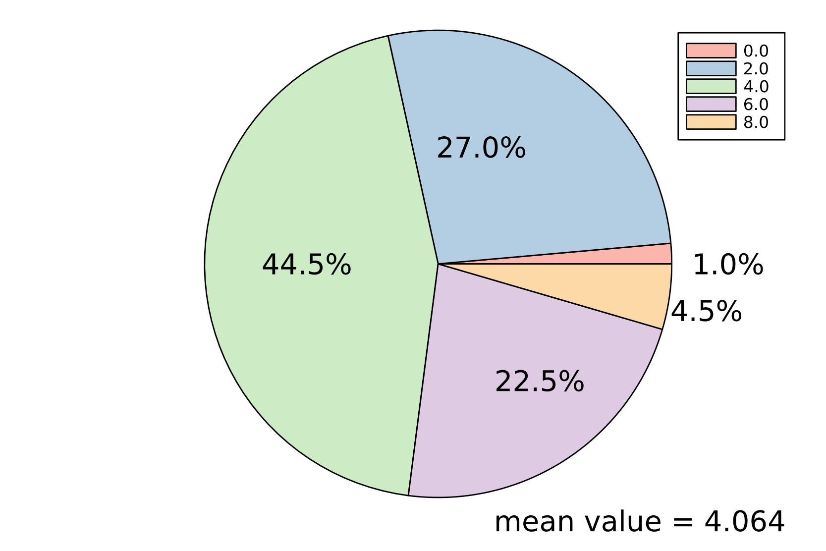
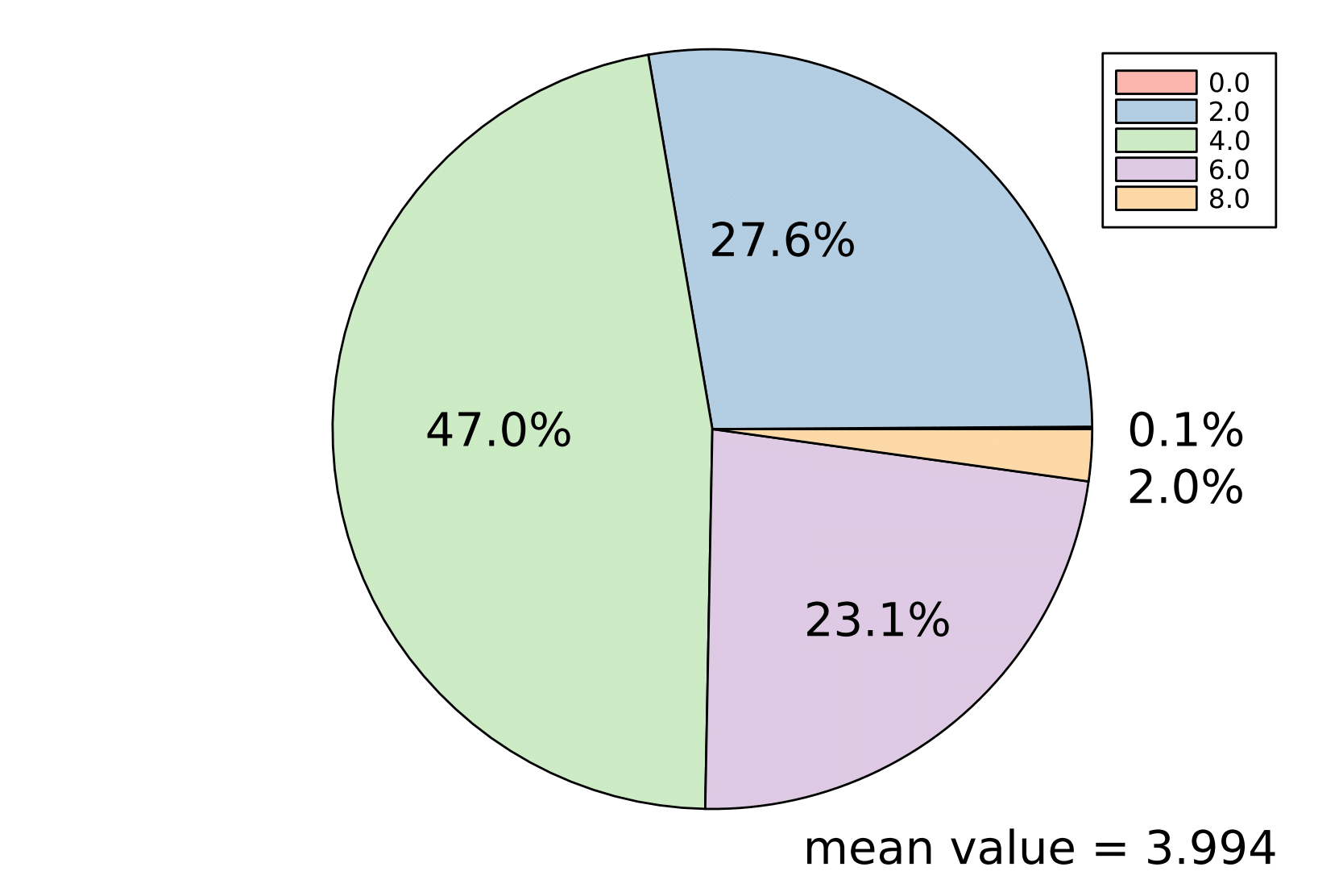
The two pie charts show the outcome of the following two experiments. We sampled \(N=1000\) random linear spaces, once with distribution \(\mathrm{Unif}(\mathbb G)\) (the left chart) and once with distribution \(\psi\) (the right chart). Then, we computed \(\mathcal E\cap L\) by solving the system of polynomial equations with the software HomotopyContinuation.jl. The charts show the empirical distribution of real zeros and the corresponding empirical means in these experiments.
Mathematica computations
We include the Mathematica computations made in Section 5.
Recall that to understand if an element \(\mathbf{x} \in \mathbb{R}^3_{\geq 0}\) belongs to the zonoid \(L\), we have to test that \(\langle \mathbf{x}, \mathbf{\rho} \rangle \leq h_L(\mathbf{\rho})\) for all \(\mathbf{\rho}\).
Now, to prove that
for \(\lambda_1=0.73, \lambda_2 = 0.86, \lambda_3 = 0.85, \lambda_4=0.966, \lambda_5 = 0.957\) we follow the procedure described below and as an example of computation let us show that \(\lambda_1(\mathbf{p}_1+\mathbf{p}_3)\in L\). Notice that
With the Mathematica command
MinValue[{Sqrt[x^2 + y^2]/(x + Pi/2*y)*EllipticE[Pi*1/2, x^2/(x^2 + y^2)],x >= 0, y >= 0},{x, y} ] // N
we compute
Therefore
hence \(\lambda_1(\mathbf{p}_1+\mathbf{p}_3)\in L\) and by symmetry also \(\lambda_2 (\mathbf{p}_1+\mathbf{p}_3)\in L\). Similarly, we find
with the following Mathematica commands:
MinValue[{Sqrt[x^2 + y^2]/(x + Pi/3*y)*EllipticE[Pi*1/2, x^2/(x^2 + y^2)], x >= 0, y >= 0},{x, y} ] // N

MinValue[{Sqrt[x^2 + y^2]/(2/3*x + Pi/2*y)*EllipticE[Pi*1/2, x^2/(x^2 + y^2)], x >= 0, y >= 0}, {x, y} ] // N

MinValue[{Sqrt[x^2 + y^2]/(x + Pi/6*y)*EllipticE[Pi*1/2, x^2/(x^2 + y^2)], x >= 0, y >= 0}, {x, y} ] // N

MinValue[{Sqrt[x^2 + y^2]/(1/3*x + Pi/2*y)*EllipticE[Pi*1/2, x^2/(x^2 + y^2)], x >= 0, y >= 0}, {x, y} ] // N
We conclude this section with the Mathematica commands used to compute \(\int_P\rho_1\cdot \rho_2\;\mathrm d\boldsymbol \rho\).
P = {{0, 0, 0}, {1, 0, 0}, {0, 1, 0}, {0, 0, 1}, 0.73*{1, 0, 1}, 0.73*{0, 1, 1}, 0.86*{0, 1, 2/3}, 0.86*{1, 0, 2/3}, 0.85*{2/3, 0, 1}, 0.85*{0, 2/3, 1}, 0.966*{1, 0, 1/3}, 0.966*{0, 1, 1/3}, 0.957*{1/3, 0, 1}, 0.957*{0, 1/3, 1}}
Conv = ConvexHullMesh[P]
Vol = Integrate[x1*x2, {x1, x2, x3} \[Element] Conv].
Project page created: 18/01/2023
Project contributors: Paul Breiding, Samantha Fairchild, Pierpaola Santarsiero, and Elima Shehu
Software used: Mathematica (version 13.0.1) and Julia (version 1.7.1)
System setup used: MacBook Pro with macOS Ventura 13.0.1, Processor 2,6 GHz 6-Core Intel Core i7, Memory 16 GB 2667 MHz DDR4, Graphics Intel UHD Graphics 630 1536 MB.
Corresponding author of this page: Pierpaola Santarsiero, pierpaola.santarsiero@mis.mpg.de