Farey polynomials
The Farey polynomials are a class of polynomials with integer coefficients (or, in the general case — known as the ‘elliptic’ case — with coefficients from the integers of an algebraic field extension of \(\mathbb{Q}\)) which give one axis of a coordinate system for the moduli space of Kleinian groups. They are also interesting as combinatorial objects in their own right, and have strong links to hypergeometric functions.
History of the Farey polynomials
Warning! This section contains references to hyperbolic geometry and low-dimensional topology. If you are interested in the combinatorics, none of this is needed to understand the rest of the page!
The original definition appears in [KS94] with corrections in [KS98]; in these papers, they appear as the traces of certain words in the parabolic Riley groups (Kleinian groups freely generated by two parabolic elements) and represent the lengths of non-boundary-parallel geodesics on four-times punctured spheres. To be more precise, they represent geodesics on the boundary at infinity of certain hyperbolic 3-manifolds; see [EMS22b] (which we wrote for the average non-expert mathematical audience). For further background on the hyperbolic geometry and the geometric interpretations of trace polynomials like these, we particularly recommend [MSW02]. Some further work on the Farey words was done by David Wright after the publication of that book [W05].
We recently extended the Keen and Series theory to allow groups generated by elliptics (the parabolic theory is just a limiting case of this), in our paper [EMS22c]. In order to understand this case, we defined a family of elliptic Farey polynomials which include the parabolic polynomials as a limiting case. We found that computing with these polynomials was a difficult business since they are defined in terms of a long word in a matrix group (so all calculations involve lots of matrix products and are slow); this motivated our study in [EMS22a] of the polynomials from a purely combinatorial point of view. In the process we found many nice number-theoretic properties of the polynomials.
Number theoretic background
We will make use of a little bit of classical number theory, from the subfield of Farey sequences; for full details see Chapter III of [HW08], or Section 3 of [EMS22a], or Chapter 7 of the highly recommended [MSW02]. Define the following Farey addition operation on \(\hat{\mathbb{Q}} := \mathbb{Q} \cup \{\infty\}\) :
Of course, this is not well-defined. In order to make it well-defined, we restrict its domain: we only allow ourselves to write \((p/q)\oplus(r/s)\) when \(|ps - qr| = \pm 1\). We call pairs of rational numbers which satisfy this condition Farey neighbours. Two remarks:
This condition implies that both summands are written in least terms (i.e. \((p,q) = (r,s) = 1\)).
Secretly, this is the determinant of a matrix in \(\mathrm{PSL}(2,\mathbb{Z})\) and in the background is an ideal triangulation of the hyperbolic plane being generated by the action of this Fuchsian group on the upper half-plane (this is the Farey triangulation of \(\mathbb{H}^2\)).
The Farey neighbour relation together with the Farey addition has beautiful number-theoretic properties (related for example to continued fractions) and geometric properties (for which we also should mention the harder monograph [ASWY07]).
For our purposes it is useful to also define an inverse operation
which is again only defined on Farey neighbours.
Combinatorial construction
We begin with the parabolic case since it is slightly easier to write down. We define a family of polynomials indexed on the positive rational numbers recursively as follows:
The recursive step is only valid when the two fractions are Farey neighbours. By the number theory alluded to in the previous section, we can get to any rational number by a chain of Farey neighbours so this is not a problem. (The procedure to do this is basically the Euclidean algorithm, so it is ‘fast’; see the material on continued fractions in [HW08] and also see Section 4.5 of [GKP94].)
These are the \((\infty,\infty)\)-Farey polynomials, or the parabolic Farey polynomials. We list a few here (which we call the parabolic Fibonacci Farey polynomials),
from Table 3 of [EMS22a]; lower down on the page we integrate some Mathematica code to generate them, and a Python package is also available on Alex Elzenaar’s GitHub
(the relevant package is farey.py). We remark that these recurrence relations in the parabolic case were known to Keen and Series (see the Remark following Corollary 4.3 of [KS94]).
p/q, \Phi_{p/q}(z)
0/1, 2 - z
1/1, 2 + z
1/2, 2 + z^2
2/3, 2 - z - 2 z^2 - z^3
3/5, 2 + z + 2 z^2 + 3 z^3 + 2 z^4 + z^5
5/8, 2 + 4 z^4 + 8 z^5 + 8 z^6 + 4 z^7 + z^8
8/13, 2 - z - 2 z^2 - 5 z^3 - 12 z^4 - 22 z^5 - 32 z^6 - 44 z^7 - 54 z^8 - 53 z^9 - 38 z^{10} - 19 z^{11} - 6 z^{12} - z^{13}
13/21, 2 + z + 2 z^2 + 7 z^3 + 14 z^4 + 31 z^5 + 64 z^6 + 124 z^7 + 214 z^8 + 339 z^9 + 498 z^{10} + 699 z^{11} + 936 z^{12} + 1148 z^{13} + 1216 z^{14} + 1064 z^{15} + 746 z^{16} + 409 z^{17} + 170 z^{18} + 51 z^{19} + 10 z^{20} + z^{21}
21/34, 2 + z^2 + 8 z^4 + 24 z^5 + 68 z^6 + 192 z^7 + 516 z^8 +1256 z^9 + 2834 z^{10} + 5912 z^{11} + 11460 z^{12} + 20816 z^{13} +  35598 z^{14} + 57248 z^{15} + 86446 z^{16} + 122560 z^{17} + 163199 z^{18} + 203952 z^{19} + 238564 z^{20} + 259704 z^{21} + 260686 z^{22} + 238320 z^{23} + 195694 z^{24} + 142328 z^{25} + 90451 z^{26} + 49552 z^{27} +  23058 z^{28} + 8952 z^{29} + 2831 z^{30} + 704 z^{31} + 130 z^{32} + 16 z^{33} + z^{34}
34/55, 2 -z - 4 z^2 - 10 z^3 - 34 z^4 - 103 z^5 - 286 z^6 - 791 z^7 - 2078 z^8 - 5221 z^9 - 12680 z^{10} - 29824 z^{11} -  67872 z^{12} - 149896 z^{13} - 321800 z^{14} - 671896 z^{15} - 1364228 z^{16} - 2692102 z^{17} - 5158232 z^{18} - 9587668 z^{19} - 17273444 z^{20} - 30141702 z^{21} - 50903644 z^{22} - 83138942 z^{23} - 131230688 z^{24} - 200056876 z^{25} - 294348624 z^{26} - 417663240 z^{27} -  571010576 z^{28} - 751328456 z^{29} - 950188464 z^{30} - 1153232920 z^{31} - 1340813030 z^{32} - 1490107333 z^{33} - 1578696308 z^{34} - 1589182962 z^{35} - 1513960786 z^{36} - 1358696535 z^{37} - 1142850158 z^{38} - 896137319 z^{39} - 651440922 z^{40} - 436582355 z^{41} - 268228504 z^{42} - 150207744 z^{43} - 76207672 z^{44} - 34797892 z^{45} - 14193584 z^{46} - 5125756 z^{47} - 1621110 z^{48} - 442809 z^{49} - 102556 z^{50} - 19630 z^{51} - 2990 z^{52} - 341 z^{53} - 26 z^{54} - z^{55}
Observe that there are already some interesting properties visible, for instance unimodularity (up to sign).
The elliptic Farey polynomials come in rationally-parameterised families which depend on two fixed parameters, \(a, b \in \mathbb{Z}\). Define \(\alpha = \exp(\pi i/a)\) and \(\beta = \exp(\pi i/b)\); then we give the three base cases of a recursive definition like that above:
The actual recursive step is slightly more complicated: the formula to get to \((p/q) \oplus (r/s)\) from \(p/q\) and \(r/s\) depends on the parity of \(q+s\). (We do not understand the geometric reason for this, and we would like to know!) Let \(p/q\) and \(r/s\) be Farey neighbours. If \(q+s\) is even, then
Otherwise if \(q + s\) is odd, then
When \(a = b = \infty\) — equivalently \(\alpha = \beta = 1\) — this reduces to the parabolic recursion relation.
A few polynomials are listed in Table 2 of [EMS22a], but a large number are found here in text format directly readable by Mathematica: fareys_general.txt.
Observations, conjectures, questions
The parabolic polynomials are unimodal (up to sign of coefficients).
There are uniform bounds for the coefficients depending only on \(q\) (this follows from a similar argument to that given in Section A.4 of [KS93])
The parabolic polynomials are essentially Tschebychev polynomials, see Section 5 of [EMS22a] and also [CEKLMR20].
Define the reduced Farey polynomials (in the parabolic case; these have nice dynamical properties, see [EMS21]) by \(\phi_{p/q}(z) = \Phi_{p/q}(z) - 2\). We conjecture that these are squares (up to multiplying by \(\pm z^{k}\) for \(k \in \{0,1\}\)); see Conjecture 3 of [EMS21] and Conjecture 6.7 of [EMS22a].
The coefficient of \(z^d\) in \(\Phi_{p/q}(z)\) is piecewise polynomial in \(d\); for a more precise conjecture, see Table 10.1 and Conjecture 10.4.2 of [E22].
The coefficients of the elliptic polynomials are Laurent polynomials in \(\alpha\) and \(\beta\). Here are some of the zero sets of these polynomials (here the rational parameters \(p/q\) are sorted in increasing absolute order, not by size of denominator; we restrict \(q \leq 10\); and the coefficient shown is the coefficient of \(z\) in each polynomial):
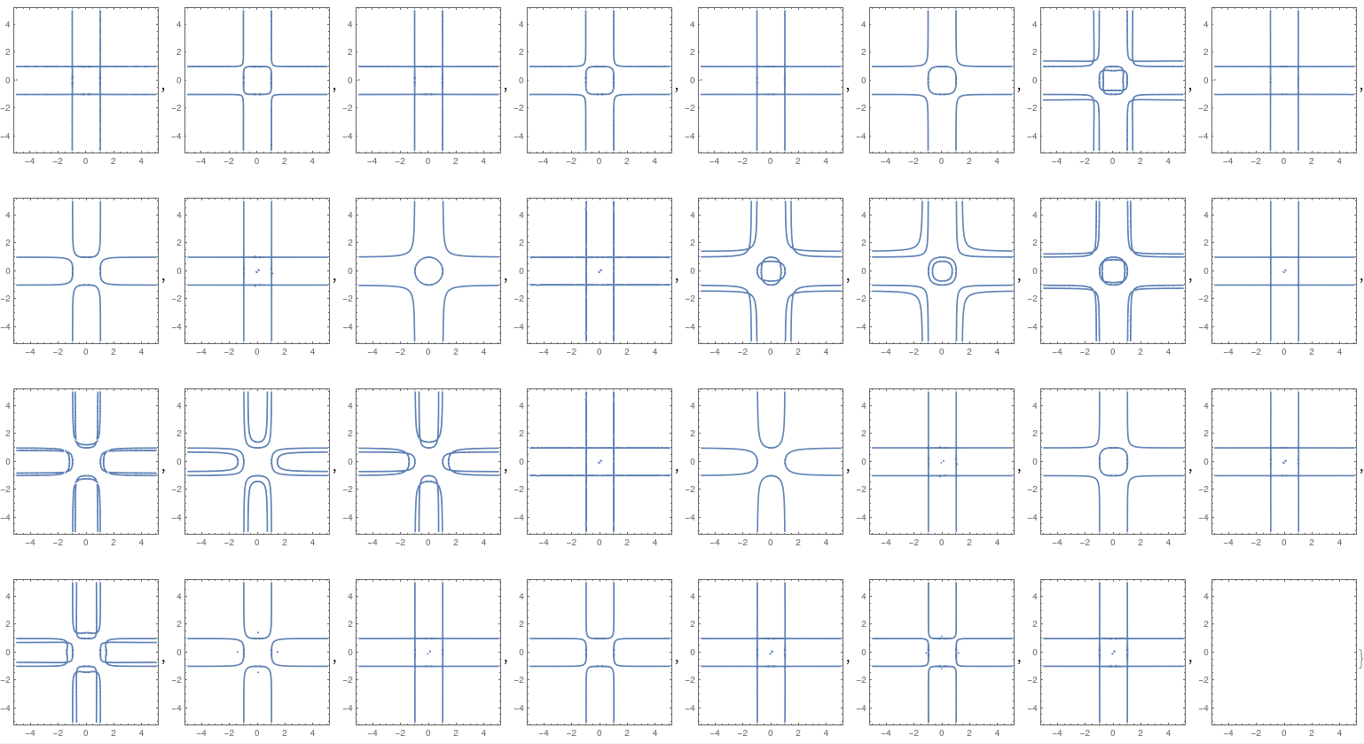
Here is the Mathematica code used to generate these plots. It needs to be run in the same directory as the file fareys_general.txt containing
the list of Farey polynomials (see Software implementations below for the relevant Mathematica code).
fareyList = << "fareys_general.txt";

fareyList =
  Sort[fareyList,
  Function[{a, b},
    a[[1]][[1]]/a[[1]][[2]] < b[[1]][[1]]/b[[1]][[2]]]];

fareyPlots =
  Map[ContourPlot[
      Coefficient[#[[2]], z] == 0, {a, -5, 5}, {b, -5, 5}] &,
    fareyList];
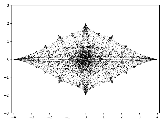
The zeros of the parabolic Farey polynomials (again with \(q \leq 10\)) accumulate to form a nice shape:

In fact this set is contained in the Riley slice exterior (essentially we proved this result in [EMS21]). For the sake of reproducibility, here is the
code (again depending on the file fareys_general.txt):
fareyList = << "fareys_general.txt";
fareyList = Map[#[[2]] &, fareyList] /. {a -> 1, b -> 1};

zeros = Map[Function[f, NSolve[f == 0, z]], fareyList];

ComplexListPlot[z /. # & /@ Flatten[zeros],
  PlotRange -> {{-4, 4}, {-2, 2}}, PlotMarkers -> {\[Bullet], 2},
  PlotStyle -> Opacity[0.5, Black], ImageSize -> 600]
Can you explain the nice patterns visible in this image? (For some results in this direction see [G08].)
In summary, we would like to know more about the coefficients (especially in the elliptic case, given the nice symmetries in \(\alpha\) and \(\beta\) which are visible in the plots and in the tables) and the factors and zeros of the Farey polynomials; we would also like to know about the dynamical properties of the recurrence relation as a dynamical system on the Farey triangulation, c.f. Section 6 of [EMS22a]. Many geometric questions may be posed and conjectures made as well, but these require more background to discuss. We have several comprehensive lists of questions:
A dynamical systems viewpoint
WANTED! Can you explain the chaos of this plot: fareytiling.pdf (generated by tiles.nb)???
This shows a dynamical system indexed by the Farey triangulation and valued in \(\mathbb{F}_3\) (hence the three colours), given by the parabolic Farey polynomial recurrence. Even though it looks globally chaotic, in many places there are clear patterns visible…
Software implementations
We have implemented the recursive definition numerically in the farey.py file of the GitHub repository https://github.com/aelzenaar/riley/, and a Mathematica file which uses the original
combinatorial group theoretic definition (c.f. Section 1 of [EMS22a]) can be downloaded here: elliptic_words.nb. This will generate all the Farey polynomials
\(\Phi^{a,b}_{p/q}(z)\) for \(q \leq 10\) (this can be changed on line 25) and output the result into fareys_general.txt (line 32) — but it is very slow! A Mathematica implementation
which produces the list of elliptic Fibonacci Farey polynomials (we listed the parabolic ones above) can be downloaded here: fibrecurse.nb This is essentially how
we produced Figure 9 of [EMS22a].
References
Hirotaka Akiyoshi, Makoto Sakuma, Masaaki Wada, and Yasushi Yamashita. Punctured torus groups and 2-bridge knot groups I. Lecture Notes in Mathematics 1909. Springer, 2007. isbn: 978-3-540-71807-9. https://doi.org/10.1007/978-3-540-71807-9.
Eric Chesebro, Cory Emlen, Kenton Ke, Denise Lafontaine, Kelly McKinnie, and Catherine Rigby. “Farey recursive functions”. In: Involve 41 (2020), pp. 439–461. https://doi.org/10.2140/involve.2021.14.439. https://arxiv.org/abs/2008.13303.
Alex Elzenaar. Deformation spaces of Kleinian groups. MSc thesis. The University of Auckland, 2022. url: https://aelzenaar.github.io/msc_thesis.pdf
Alex Elzenaar, Gaven Martin, and Jeroen Schillewaert. “Approximations of the Riley slice.” November 2021. https://arxiv.org/abs/2111.03230 [math.GT].
Alex Elzenaar, Gaven Martin, and Jeroen Schillewaert. “The combinatorics of the Farey words and their traces.” April 2022. https://arxiv.org/abs/2204.08076 [math.GT]. Slightly updated version available at url: https://aelzenaar.github.io/farey/farey.pdf
Alex Elzenaar, Gaven Martin, and Jeroen Schillewaert. “Concrete one complex dimensional moduli spaces of hyperbolic manifolds and orbifolds”. In: 2021-22 MATRIX annals. Ed. by David R. Wood, Jan de Gier, Cheryl E. Prager, and Terrence Tao. MATRIX Book Series 5. Springer, to appear. https://arxiv.org/abs/2204.11422 [math.GT].
Alex Elzenaar, Gaven Martin, and Jeroen Schillewaert. “The Riley slice and its elliptic cousins.” To appear.
Ronald L. Graham, Donald E. Knuth, and Oren Patashnik. Concrete mathematics. A foundation for computer science. 2nd ed. Addison-Wesley, 1994.
Jane Gilman. “The structure of two-parabolic space: parabolic dust and iteration”. In: Geometriae Dedicata 131 (2008), pp. 27–48. https://doi.org/10.1007/s10711-007-9215-z
Godfrey H. Hardy and Edward M. Wright. An introduction to the theory of numbers. Revised by D. R. Heath-Brown and J. H. Silverman. 6th ed. Oxford University Press, 2008. isbn: 978-0-19-921985-8.
Linda Keen and Caroline Series. “Pleating coordinates for the Maskit embedding of the Teichmüller space of punctured tori”. In: Topology 32.4 (1993), pp. 719–749. https://doi.org/10.1016/0040-9383(93)90048-z
Linda Keen and Caroline Series. “The Riley slice of Schottky space”. In: Proceedings of the London Mathematics Society 3.1 (69 1994), pp. 72–90. https://doi.org/10.1112/plms/s3-69.1.72
Yohei Komori and Caroline Series. “The Riley slice revisited”. In: The Epstein birthday schrift. Ed. by Igor Rivin, Colin Rourke, and Caroline Series. Geometry and Topology Monographs 1. Mathematical Sciences Publishers, 1998, pp. 303–316. https://doi.org/10.2140/gtm.1998.1.303. https://arxiv.org/abs/math/9810194
David Mumford, Caroline Series, and David Wright. Indra’s pearls. The vision of Felix Klein. Cambridge University Press, 2002. isbn: 0-521-35253-3.
David Wright. “Searching for the cusp”. In: Spaces of Kleinian groups. Ed. by Yair N. Minsky, Makoto Sakuma, and Caroline Series. LMS Lecture Notes 329. Cambridge University Press, 2005, pp. 301–336. https://doi.org/10.1017/cbo9781139106993.016.
Project page created: 06/05/2022
Project contributors: Alex Elzenaar, Gaven Martin, Jeroen Schillewaert.
Corresponding author of this page: Alex Elzenaar, https://aelzenaar.github.io/ mailto:elzenaar@mis.mpg.de
Software used: Mathematica 12.1