Logarithmic Voronoi cells

In this notebook, we present computations from the article Logarithmic Voronoi cells available at https://arxiv.org/abs/2006.09431. We quote from the beginning of that article now.

For any subset \(X \subset \mathbb{R}^n\), the Voronoi cell of a point \(p \in X\) consists of all points of \(\mathbb{R}^n\) which are closer to \(p\) than to any other point of \(X\) in the Euclidean metric. In this article we discuss the analogous logarithmic Voronoi cells which find application in statistics. A discrete statistical model is a subset of the probability simplex \(\mathcal{M} \subset \Delta_{n-1}\), since probabilities are positive and sum to \(1\). The maximum likelihood estimator \(\Phi\) (MLE) sends an empirical distribution \(u \in \Delta_{n-1}\) of observed data to the point in the model which best explains the data. This means \(p = \Phi(u)\) maximizes the log-likelihood function \(\ell_u(p) := \sum_{i=1}^n u_i \log(p_i)\) restricted to \(\mathcal{M}\). Note that \(\ell_u\) is strictly concave on \(\Delta_{n-1}\) and takes its maximum value at \(u\). Usually, \(u \notin \mathcal{M}\), and we must find the point \(\Phi(u) \in \mathcal{M}\) which is closest in the log-likelihood sense. For \(p \in \mathcal{M}\) we define the logarithmic Voronoi cell

\[\log \text{Vor}_\mathcal{M}(p) := \left\{ u \in \Delta_{n-1} : \Phi(u) = p \right\}.\]

Information Geometry considers MLE in the context of the Kullbach-Leibler divergence of probability distributions, sending data to the nearest point with respect to a Riemannian metric on \(\Delta_{n-1}\). Algebraic Statistics considers the case where \(\mathcal{M}\) can be described as either the image or kernel of algebraic maps. Recent work in Metric Algebraic Geometry concerns the properties of real algebraic varieties that depend on a distance metric. Logarithmic Voronoi cells are natural objects of interest in all three subjects.

The computation in this notebook

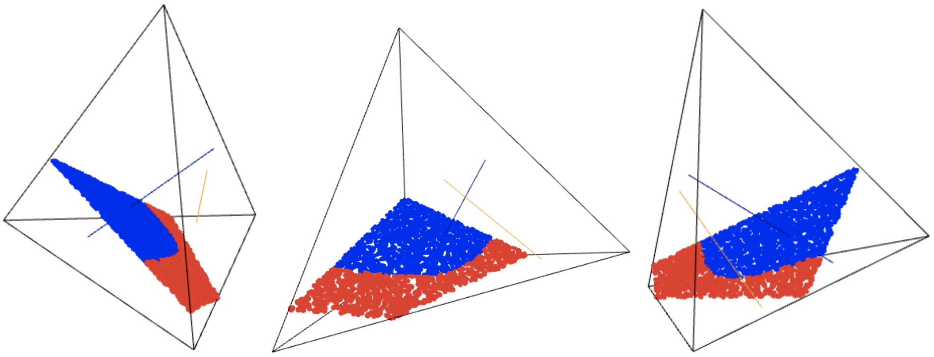
One result of that article states that, for linear models, the logarithmic Voronoi cells are always polytopes. One might hope that finite unions of linear models would admit logarithmic Voronoi cells which are polytopes. However, this is not the case. The log-normal spaces from two disjoint linear models can meet in such a way that the boundary created on a logarithmic Voronoi cell is nonlinear. For an explicit example with two linear models, \(\mathcal{M} := \mathcal{M}_1 \cup \mathcal{M}_2 \subset \Delta_3 \subset \mathbb{R}^4\), we present the computations in this notebook. Here

\[\begin{split}\mathcal{M}_1 = \left\{ (1-s)p_1 + s p_2 \, : \, s \in [0,1] \subset \mathbb{R} \right\},\\ \mathcal{M}_2 = \left\{ (1-t)q_1 + t q_2 \, : \, t \in [0,1] \subset \mathbb{R} \right\},\\ p_1 = (1/5,1/5,3/5,0),\\ p_2 = (1/7,3/7,0,3/7),\\ q_1 = (1/13,9/13,3/13,0),\\ q_2 = (4/13,4/13,0,5/13).\end{split}\]

We sampled \(3000\) points from the log-normal polytope of a given point

\[p = (19/105, 29/105, 2/5, 1/7) \in \mathcal{M}_1\]

and colored them blue or red depending on if their MLE was \(p\) or if their MLE was located on \(\mathcal{M}_2\). Therefore, the blue convex set produced below is the logarithmic Voronoi cell of \(p \in \mathcal{M}\).

# some points to create linear models by the line which is their affine span
p1 = vector([1/5,1/5,3/5,0])
p2 = vector([1/7,3/7,0,3/7])
q1 = vector([1/13,9/13,3/13,0])
q2 = vector([4/13,4/13,0,5/13])

s,t = var('s t') # variables for parametrizing our linear models
assume(s>0, t>0, s<1, t<1)
x = (1-s)*p1 + s*p2 # the first linear model M_1
y = (1-t)*q1 + t*q2 # the second linear model M_2
yprime = derivative(y,t) # we will need these derivatives later to compute the MLE

xchosen = x.subs(s=1/3)
xchosen

(19/105, 29/105, 2/5, 1/7)

Now we find the equation of the log-normal space at the chosen point xchosen \(\in \mathcal{M}_1\).

v = p2 - p1 # direction vector for M_1 linear model
V = matrix(4,1,v)
LN = V.left_kernel().basis_matrix() # equations defining the same model

uvarz = [var('u%s'%i) for i in [1..4]]
LN = LN.change_ring(SR)
Aaugmented = LN.T.augment(vector([ uvarz[i] / xchosen[i] for i in range(4) ]))
deter = det(Aaugmented)
deter # this defines the log-normal space at the point xchosen

-14/19*u1 + 56/29*u2 - 7/2*u3 + 7*u4

Below we find a basis for the two-dimensional log-normal space. We will use this basis to sample from the log-normal polytope of the point xchosen \(\in \mathcal{M}_1\).

rowz = [[1,1,1,1], [deter.coefficient(uvar) for uvar in uvarz]]
B = matrix(rowz)
RN = B.right_kernel_matrix()
C = RN.T
C

[     1      0]
[     0      1]
[-14/19 -14/29]
[ -5/19 -15/29]

Here we use rejection sampling to fill the log-normal polytope at xchosen with sample points. Later we will color each point blue or red.

T = RealDistribution('uniform', [-0.9, 0.9])
def rejectionsample(xchosen, C, N):
    samplez = []
    while len(samplez) < N:
        w = vector([T.get_random_element(),T.get_random_element()])
        sample = vector(xchosen) + C * w
        okay = True
        for entry in sample:
            if entry < 0:
                okay = False
            if entry > 1:
                okay = False
        if okay:
            samplez.append(sample)
    return samplez

samplez = rejectionsample(xchosen, C, 3000)
print(len(samplez), samplez[0] )

3000 (0.055162043665491406, 0.5018003023939119, 0.383772528436231, 0.059265125504365745)

Here we define the log-likelihood function \(\ell_u(p) := \sum u_i log(p_i)\). Then we define a function to compute the MLE of a given sample point according to the model \(\mathcal{M}_2\). We will compare these values with \(\ell_u(\) xchosen \()\).

def ell(u,p):
    # compute \ell_u(p) log-likelihood function based at data point u, for point in model p \in M.
    return sum([u[i]*(log(p[i]).n()) for i in range(len(u))])

def computeMLE(sample):
    eqn = sum([sample[i]/y[i] * yprime[i] for i in range(len(y))])
    eqn = (eqn*eqn.denominator()).rational_simplify()
    tstar = RDF(find_root(eqn,0,1))
    return ell(sample, y.subs(t=tstar))

# for plotting 4-dimensional vectors in 3-dimensional hyperplane
Q,R = matrix(RDF,4,1,[1,1,1,1]).QR()

Here we run through all our sample points, and compare the values of \(\ell_u(\) xchosen \()\) against the maximum value of \(\ell_u(q)\) where \(q \in \mathcal{M}_2\). If \(\ell_u(\) xchosen \()\) is larger, then we color the point blue. Otherwise, we color the point red.

plt2 = Graphics()
pp1 = (Q.T * p1)[1:len(p1)]
pp2 = (Q.T * p2)[1:len(p1)]
qq1 = (Q.T * q1)[1:len(p1)]
qq2 = (Q.T * q2)[1:len(p1)]
verts = [vector([1,0,0,0]), vector([0,1,0,0]), vector([0,0,1,0]), vector([0,0,0,1])]
verts = [(Q.T * vert)[1:len(p1)] for vert in verts]
for vtup in [(verts[0],verts[1]), (verts[0],verts[2]), (verts[0],verts[3]),
            (verts[1],verts[2]), (verts[1],verts[3]),
            (verts[2],verts[3])]:
    v1,v2 = vtup[0],vtup[1]
    plt2 += line([v1,v2],color='black',thickness=2)
plt2 += line([pp1,pp2],color='darkblue',thickness=15)
plt2 += line([qq1,qq2],color='orange',thickness=15)
for pt in samplez:
    pt3d = (Q.T * pt)[1:len(pt)]
    MLEoriginal = ell(pt, xchosen)
    clr = 'blue'
    if computeMLE(pt) > MLEoriginal:
        clr = 'red'
    plt2 += point(pt3d, color=clr)

We output our sampling of the logarithmic Voronoi cell of xchosen viewed as an element of \(\mathcal{M} = \mathcal{M}_1 \cup \mathcal{M}_2\). This demonstrates the nonlinear boundary that can be created when the model is a disjoint union of linear models. The blue convex set pictured below is the logarithmic Voronoi cell. If you run this Jupyter notebook yourself, the next cell with show(plt2, frame=False) would output an interactive 3d image which can be rotated and zoomed to various viewpoints.

show(plt2, frame=False)

In case the interactive 3-dimensional display above malfunctions, we include three viewpoints in a static image file below.