Maximal Mumford Curves from Planar Graphs
Abstract: A curve of genus \(g\) is maximal Mumford (MM) if it has \(g+1\) ovals and \(g\) tropical cycles. We construct full-dimensional families of MM curves in the Hilbert scheme of canonical curves. This rests on first-order deformations of graph curves whose graph is planar.
We implemented an algorithm that computes the tangent cone of first order deformations of a graph curve that lift to MM-curves. We provide a complete list of these tangent cones for graph curves of small genus. We also provide code computing the number of connected components of a real curve, which we used for numerical confirmations.
The MM-Cone
Let \(C_G \subset \mathbb{P}^{g-1}\) be a graph curve whose dual graph \(G\) is a planar trivalent graph of genus \(g\) with \(2g-2\) vertices. For any edge pairing \(\rho\) of \(G\), the tangent space to the Hilbert scheme at \(C_G\) contains a full-dimensional open cone
of first order deformations of \(C_G\) that lift to smooth curves whose topology corresponds to \(\rho\).
We implemented an algorithm that inputs a graph \(G\) and an edge pairing \(\rho\), and outputs a basis for the \(\mathbb{R}_{>0}^{3g-3}\) factor of the corresponding tangent cone.
The Macaulay2 code can be downloaded here: tangent-directions.m2.
The MM-cone refers to this tangent cone when the edge pairing \(\rho\) comes from the unique double cover of \(G\) by \(g+1\) cycles. In this case, the first order deformations in our cone lift to MM-curves.
Example:
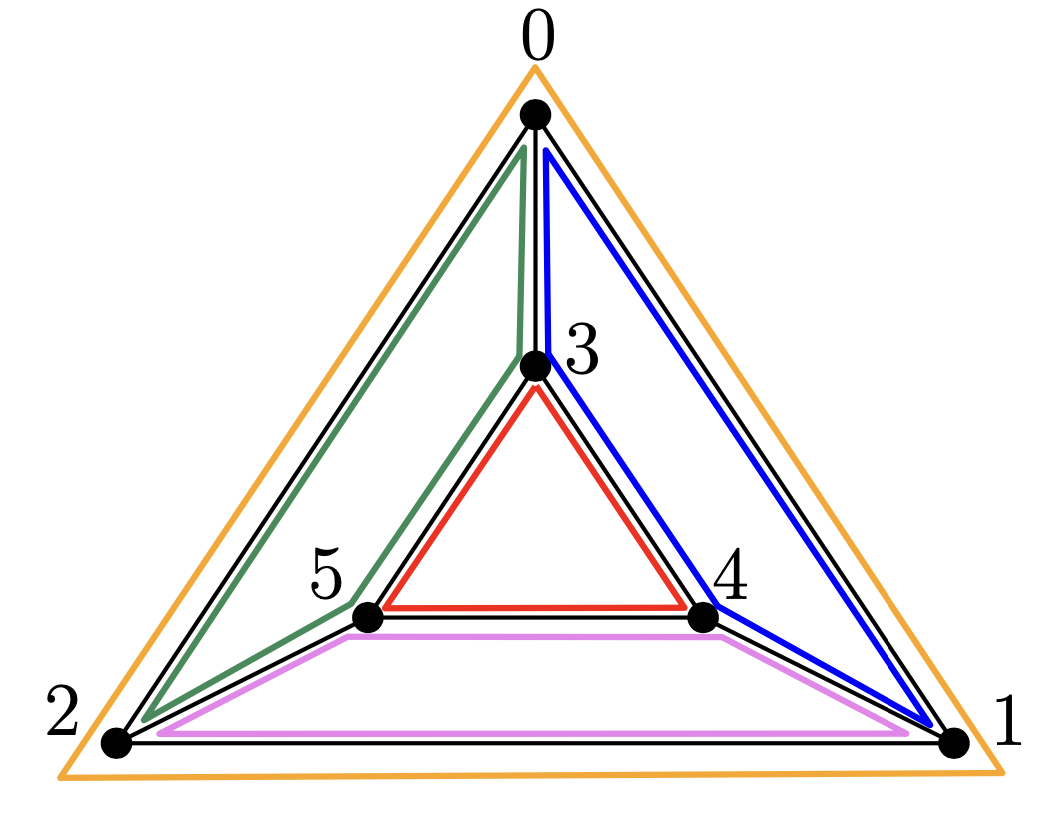
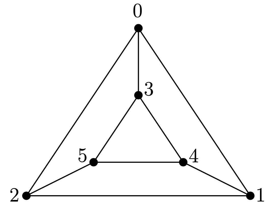
Here, we explain an example of input and output from our algorithm. Consider the following planar trivalent graph \(G\) of genus \(4\), and its double cover by its \(5\) face cycles.
The input is the list of edges of our graph \(G\) and the edge pairing corresponding to the double cover above.
Per our paper, an edge pairing \(\rho\) is defined as follows: for every edge \(e = \{i,j\}\) with adjacent edges \(e_i, e_i'\) and \(e_j, e_j'\), respectively, \(\rho(e)\) is a partition of these four adjacent edges into either
In our code, such a partition \(\rho(e)\) is encoded via either one of the pairs in it. Thus, an edge pairing \(\rho\) is encoded as a list of pairs \(\rho(e)\), where the order of the edges \(e\) is the same as in the inputted list of edges of the graph.
The edge pairing associated to the double cover above is the one where each \(\rho(e)\) contains edges belonging to the same face cycle of \(G\).
Edges = {{0,1}, {1,2}, {2,0}, {3,4}, {4,5}, {5,3}, {0,3}, {1,4}, {2,5}};

EdgePairing = {{1,2}, {0,2}, {0,1}, {4,5}, {3,5}, {3,4}, {2,5}, {1,4}, {1,4}};
The output is:
A list \(L\) of generators of the ideal \(I \subset S:= \mathbb{Q}[x_0, x_1,\dots, x_{g-1}]\) of the graph curve \(C_G\).
A list of \(3g-3\) tangent directions \(\eta_e\), where each \(\eta_e\) deforms the node of \(C_G\) corresponding to the edge \(e\) according to the inputted edge pairing. Each tangent vector is thought of as an element of \(\operatorname{Hom}_S(I, S/I)_0\) and is encoded as a list of size \(\#L\).
The sum \(\eta\) of all the tangent vectors \(\eta_e\), which is a vector in the interior of our MM-cone.
Generators of graph curve ideal:
{x_0^2+x_0*x_1+x_0*x_2+x_0*x_3, x_1*x_2*x_3}

Tangent vectors:
matrix {{0, x_0*x_1^2},
        {0, x_0*x_2^2},
        {0, x_0*x_3^2},
        {0, -x_0*x_1^2-x_1^3-x_1^2*x_2-x_1^2*x_3},
        {0, -x_0*x_2^2-x_1*x_2^2-x_2^3-x_2^2*x_3},
        {0, -x_0*x_3^2-x_1*x_3^2-x_2*x_3^2-x_3^3},
        {-x_1*x_3, 0},
        {-x_1*x_2, 0},
        {-x_2*x_3, 0}}

Sum of tangent vectors:
{-x_1*x_2-x_1*x_3-x_2*x_3,
 -x_1^3-x_1^2*x_2-x_1*x_2^2-x_2^3-x_1^2*x_3-x_2^2*x_3-x_1*x_3^2-x_2*x_3^2-x_3^3}
The first order deformation of \(C_G\) along \(\eta\) lifts to an MM-curve.
How to determine the MM edge pairing?
Consider any planar trivalent \(3\)-connected graph \(G\) of genus \(g\). The graph \(G\) admits a unique double cover by \(g+1\) cycles via its face cycles (including the outer rim).
As above, the MM-cone corresponds to the edge pairing \(\rho\) where each pair \(\rho(e)\) belongs to the same face cycle. Thus, the edge pairing that gives the MM-cone can be read easily from any planar embedding of our graph \(G\).
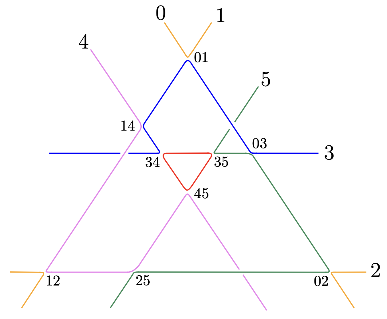
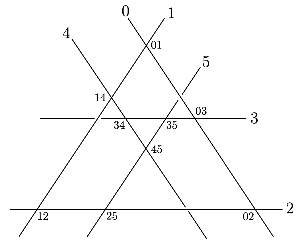
The function tutte_lifting in polymake provides such a planar embedding when \(G\) contains a \(3\)-cycle.
Since our graphs are always trivalent, one can introduce a \(3\)-cycle by replacing a vertex by a \(3\)-cycle.
$edges = [[0,1], [1,2], [2,0], [3,4], [4,5], [5,3], [0,3], [1,4], [2,5]];

$G = graph_from_edges($edges);

$T = tutte_lifting($G);

print $T->VISUAL;
Data for Low Genus
There are \(1\), \(2\), \(4\), \(14\), and \(57\) trivalent \(3\)-connected graphs of genus \(3\), \(4\), \(5\), \(6\), and \(7\), respectively.
Out of these graphs, \(1\), \(1\), \(2\), \(5\), and \(14\), respectively, are planar.
We ran our code and computed the MM-cones for all these planar graphs.
The input/output data can be downloaded here: mm-cones-low-genus.txt.
Numerical Confirmations
We used numerical methods to confirm that our lifts have the expected number of connected components.
We used code written by Jonathan Hauenstein that computes the number of connected components of a complete intersection of three hypersurfaces in \(\mathbb{RP}^4\).
The code runs in MATLAB and calls Bertini.
It can be downloaded here: connectivity-computation.zip.
For another numerical approach to computing the connectivity of a smooth algebraic curve, using gradient flows, see the article Smooth connectivity in real algebraic varieties by Cummings, Hauenstein, Hong, and Smyth.
Example:
Continuing the previous example, we check numerically that the smooth genus \(4\) lift \(V(I + t * \eta) \subset \mathbb{P}^3\) has \(5\) connected components, hence is maximal, for small \(t\).
For input, set:
the parameter \(t\) in the file \(\text{runTest.m}\), and
the three equations cutting out the curve and their total derivatives in the files \(\text{input_slice}\) and \(\text{input_crit}\). (In our example, the third equation simply cuts out a hyperplane \(\mathbb{P}^3 \subset \mathbb{P}^4\).)
f1 = w * (w + x + y + z) + t * (- x * y - x * z - y * z);

f2 =  x * y * z
    + t * (- x^3 - x^2 * y - x * y^2 - y^3 - x^2 * z - y^2 * z - x * z^2 - y * z^2 - z^3);

f3 = v;


g1 =  l1 * (2*w + x + y + z) + l2 * (w - t * (y + z))
    + l3 * (w - t * (x + z)) + l4 * (w - t * (x + y));

g2 =  l2 * (y*z - t * (3*x^2 + y^2 + z^2 + 2*x*y + 2*x*z))
    + l3 * (x*z - t * (x^2 + 3*y^2 + z^2 + 2*x*y + 2*y*z))
    + l4 * (x*y - t * (x^2 + y^2 + 3*z^2 + 2*x*z + 2*y*z));

g3 = l0;
To run the code, follow these steps in MATLAB:
Set
ParameterHomotopyto \(1\) in the file \(\text{input_slice}\), and run
system('bertini input_slice');
Copy the file \(\text{start_parameters}\) to \(\text{start_parameters_slice}\) and the file \(\text{finite_solutions}\) to \(\text{start_slice}\).
Set
ParameterHomotopyback to \(2\).Repeat these three steps for \(\text{slice}\) replaced by \(\text{crit}\).
Finally, running runTest outputs the number of connected components of our real curve:
Number of connected components: 5