Algebraic Sparse Factor Analysis
Abstract: Factor analysis is a statistical technique that explains correlations among observed random variables with the help of a smaller number of unobserved factors. In traditional full factor analysis, each observed variable is influenced by every factor. However, many applications exhibit interesting sparsity patterns, that is, each observed variable only depends on a subset of the factors. In this paper, we study such sparse factor analysis models from an algebro-geometric perspective. Under mild conditions on the sparsity pattern, we examine the dimension of the set of covariance matrices that corresponds to a given model. Moreover, we study algebraic relations among the covariances in sparse two-factor models. In particular, we identify cases in which a Groebner basis for these relations can be derived via a 2-delightful term order and joins of toric edge ideals.
Supplementary Material
This page contains supplementary material for the computations performed in the article. The script is ending with .m2 and is run in \(\verb|Macaulay2|\). We provide code to compute the ideal of invariants for a sparse factor analysis model. First, download the file utils.m2 and run your Macaulay2 in the same folder. Then you can simply start with input "utils.m2" and
loadPackage "PhylogeneticTrees" to experiment with the functions of the script. The examples of Section 4 can be reproduced with examples.m2.
Functions
The main functions in the script are:
getIdeal(LambdaAdjMatrix): Computes an ideal based on the given coefficient matrix.circularOrderRing(p): Creates a ring with a circular term order where p is the number of observable nodes.Lambda2Digraph(LambdaAdjMatrix): Converts the coefficient matrix to a directed graph.
The following are only for the models with two latent nodes, in particular for Section 4:
getProposedIdeal(LambdaAdjMatrix): Computes the ideal generated by \((m+1) \times (m+1)\)-minors and the separation ideal.getLambda(p, k, r): Returns the coefficient matrix where \(p\) is the total number of observed variables, \(\{1,\ldots,k\}\) are the children of the first factor and \(\{p-r+1,...,p\}\) are the children of the second factor.
Socio-economic study: sparse factor insights
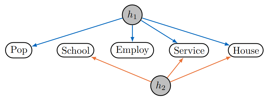
Let us look at the figure on the left: this is a (factor analysis) graph corresponding to a sparse factor analysis model for a study in which several districts in the greater Los Angeles area are considered. Two gray nodes correspond to latent variables. The study contains five socio-economic observed variables: Total population, median school years, total employment, miscellaneous professional services, and median house value. The data consists of records of twelve districts from which a covariance matrix is calculated. The sparsity pattern corresponding to the graph corresponds to the following coefficient matrix (or adjacency matrix with weights)
\(\Lambda = \begin{pmatrix}\lambda_{11} & 0 \\ 0 & \lambda_{22} \\ \lambda_{31} & 0 \\ \lambda_{41} & \lambda_{42} \\ \lambda_{51} & \lambda_{52} \end{pmatrix}\).
The graph implies, for example, that total population is independent of total employment given only the first hidden variable. Moreover, the coefficients \(\lambda_{vh}\) can be understood as the strength of causal effects that the latent variables have on the observed variables.
p=5;
LambdaAdjMatrix = matrix{{1,0},{0,1},{1,0},{1,1},{1,1}};
R = circularOrderRing(p);
I = getIdeal(matrix{{1,0},{0,1},{1,0},{1,1},{1,1}});
I = sub(I,R);
J = getProposedIdeal(LambdaAdjMatrix);
J = sub(J,R);
I == J;
The ideal is toric and its generators consist of two monads and one tetrad.
Computing the ideal of invariants of a sparse factor analysis model
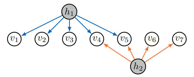
On the right, we have another example of a sparse 2-factor analysis graph. Since this is a sparse 2-factor analysis model, we can use the following:
LambdaAdjMatrix = getLambda(7, 5, 4);
I = getProposedIdeal(LambdaAdjMatrix);
In the following we show that its ideal of invariants is join of two toric ideals \(I_1\) and \(I_2\) (joinIdeal(I1,I2)) that are associated to two sparse 1-factor analysis graphs. The input joinOfInitial == initialOfJoin checks if the Gröbner basis with respect to the chosen circular order is 2-delightful.
p=7;
I1 = getIdeal(matrix{{1},{1},{1},{1},{1},{0},{0}});
I2 = getIdeal(matrix{{0},{0},{0},{1},{1},{1},{1}});
R = circularOrderRing(p);
I1 = sub(I1,R);
I2 = sub(I2,R);
I1 = ideal gens gb I1;
I2 = ideal gens gb I2;

joinOfInitial = joinIdeal(ideal(leadTerm(I1)), ideal(leadTerm(I2)));
J = joinIdeal(I1,I2);
J = sub(J,R);
J = ideal gens gb J;

initialOfJoin = ideal(leadTerm(J));
joinOfInitial == initialOfJoin;