Minimality of tensors of fixed multilinear rank

As a (very) special case of the main theorem of https://arxiv.org/abs/2007.08909, the set of \(2\times 2\) matrices of rank \(1\) is a minimal submanifold of \(\mathbb{R}^4\) under the Frobenius norm. Minimal submanifolds are a mathematical model of soap films, since they locally minimize volume given a fixed boundary. A minimal submanifold can be defined by the requirement that its mean curvature vector field be everywhere vanishing. In fact, the set of all tensors of any fixed multilinear rank forms a minimal submanifold of its ambient Euclidean space, which yields \(2 \times 2\) matrices of rank one as the special case we examine computationally in this notebook.

First, we will see a mean curvature vector field which is not everywhere vanishing. We accomplish this by examining the set of \(2 \times 2\) matrices of rank one, whose entries are required to sum to one. This set is of interest in statistics, for example, and will not be a minimal submanifold, as we will visually see.

To begin, we use a local parametrization of the set \(\mathcal{M}\) of matrices whose rank is one, and whose entries sum to one.

u1,u2 = var('u1 u2')
x = vector([u1*u2, u1*(1-u2), u2*(1-u1), (1-u1)*(1-u2)])
show(x)

$$\newcommand{\Bold}[1]{\mathbf{#1}}\left(u_{1} u_{2},\,-u_{1} {\left(u_{2} - 1\right)},\,-{\left(u_{1} - 1\right)} u_{2},\,{\left(u_{1} - 1\right)} {\left(u_{2} - 1\right)}\right)$$

sum(x).expand()

1

Below we calculate a basis for the tangent space of \(\mathcal{M}\) from our local parametrization. We also calculate the Gram matrix \(G\) in the basis coming from our local parametrization.

v1 = derivative(x,u1)
v2 = derivative(x,u2)

a11 = derivative(v1,u1)
a12 = derivative(v1,u2)
a21 = derivative(v2,u1)
a22 = derivative(v2,u2)

G = matrix(2,2,[v1.dot_product(v1), v1.dot_product(v2), v2.dot_product(v1), v2.dot_product(v2)])
show(G)

$$\newcommand{\Bold}[1]{\mathbf{#1}}\left(\begin{array}{rr} 2 \, {\left(u_{2} - 1\right)}^{2} + 2 \, u_{2}^{2} & {\left(u_{1} - 1\right)} {\left(u_{2} - 1\right)} + u_{1} {\left(u_{2} - 1\right)} + {\left(u_{1} - 1\right)} u_{2} + u_{1} u_{2} \\ {\left(u_{1} - 1\right)} {\left(u_{2} - 1\right)} + u_{1} {\left(u_{2} - 1\right)} + {\left(u_{1} - 1\right)} u_{2} + u_{1} u_{2} & 2 \, {\left(u_{1} - 1\right)}^{2} + 2 \, u_{1}^{2} \end{array}\right)$$

Below we calculate the second derivative vectors, and project them onto the normal space of \(\mathcal{M}\).

V2 = v2 - v2.dot_product(v1)*v1/v1.dot_product(v1) # orthogonalize our tangent space basis...

proja11 = a11 - a11.dot_product(v1)*v1/v1.dot_product(v1) - a11.dot_product(V2)*V2/V2.dot_product(V2)
proja12 = a12 - a12.dot_product(v1)*v1/v1.dot_product(v1) - a12.dot_product(V2)*V2/V2.dot_product(V2)
proja21 = a21 - a21.dot_product(v1)*v1/v1.dot_product(v1) - a21.dot_product(V2)*V2/V2.dot_product(V2)
proja22 = a22 - a22.dot_product(v1)*v1/v1.dot_product(v1) - a22.dot_product(V2)*V2/V2.dot_product(V2)

Below, the mean curvature vector \(h\) is calculated using the inverse of the Gram matrix and the projections of the second derivative vectors onto the normal space. We print out the first entry of the vector \(h\) to show that it is evidently nonzero. This proves that \(\mathcal{M}\) is not a minimal submanifold.

Ginv = G.inverse()
h = Ginv[0,0]*proja11 + Ginv[0,1]*proja12 + Ginv[1,0]*proja21 + Ginv[1,1]*proja22

entry = h[0]
print(entry.expand().full_simplify().expand()) # the only observation is that it is nonzero

16*u1^2*u2/(16*u1^4 + 32*u1^2*u2^2 + 16*u2^4 - 32*u1^3 - 32*u1^2*u2 - 32*u1*u2^2 - 32*u2^3 + 40*u1^2 + 32*u1*u2 + 40*u2^2 - 24*u1 - 24*u2 + 9) + 16*u1*u2^2/(16*u1^4 + 32*u1^2*u2^2 + 16*u2^4 - 32*u1^3 - 32*u1^2*u2 - 32*u1*u2^2 - 32*u2^3 + 40*u1^2 + 32*u1*u2 + 40*u2^2 - 24*u1 - 24*u2 + 9) - 8*u1^2/(16*u1^4 + 32*u1^2*u2^2 + 16*u2^4 - 32*u1^3 - 32*u1^2*u2 - 32*u1*u2^2 - 32*u2^3 + 40*u1^2 + 32*u1*u2 + 40*u2^2 - 24*u1 - 24*u2 + 9) - 40*u1*u2/(16*u1^4 + 32*u1^2*u2^2 + 16*u2^4 - 32*u1^3 - 32*u1^2*u2 - 32*u1*u2^2 - 32*u2^3 + 40*u1^2 + 32*u1*u2 + 40*u2^2 - 24*u1 - 24*u2 + 9) - 8*u2^2/(16*u1^4 + 32*u1^2*u2^2 + 16*u2^4 - 32*u1^3 - 32*u1^2*u2 - 32*u1*u2^2 - 32*u2^3 + 40*u1^2 + 32*u1*u2 + 40*u2^2 - 24*u1 - 24*u2 + 9) + 16*u1/(16*u1^4 + 32*u1^2*u2^2 + 16*u2^4 - 32*u1^3 - 32*u1^2*u2 - 32*u1*u2^2 - 32*u2^3 + 40*u1^2 + 32*u1*u2 + 40*u2^2 - 24*u1 - 24*u2 + 9) + 16*u2/(16*u1^4 + 32*u1^2*u2^2 + 16*u2^4 - 32*u1^3 - 32*u1^2*u2 - 32*u1*u2^2 - 32*u2^3 + 40*u1^2 + 32*u1*u2 + 40*u2^2 - 24*u1 - 24*u2 + 9) - 6/(16*u1^4 + 32*u1^2*u2^2 + 16*u2^4 - 32*u1^3 - 32*u1^2*u2 - 32*u1*u2^2 - 32*u2^3 + 40*u1^2 + 32*u1*u2 + 40*u2^2 - 24*u1 - 24*u2 + 9)

# special points zero mean curvature
subz = {u1:1/2, u2:1/3}
h.subs(subz)

(0, 0, 0, 0)

# most points have nonzero mean curvature vectors
subz = {u1:1/4, u2:1/5}
h.subs(subz)

(-1800/3703, 5400/25921, 6600/25921, 600/25921)

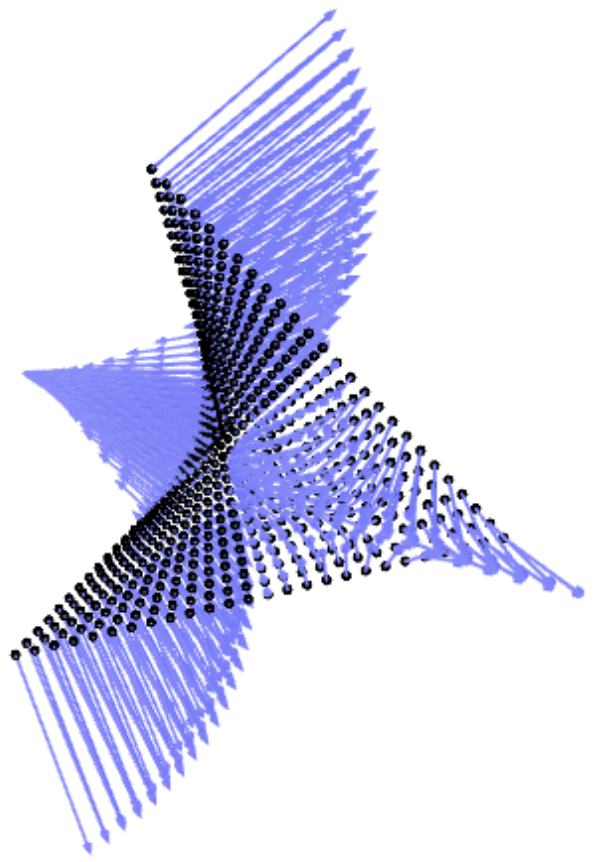
Now we can take a look at the mean curvature vector field at various points along \(\mathcal{M} \subset \mathbb{R}^4\) by projecting the entire picture onto the affine hyperplane \(P \subset \mathbb{R}^4\) where \(P = \{ x \in \mathbb{R}^4 : \sum_{i=1}^4 x_i = 1 \}\).

Q,_ = matrix(RDF,4,1,[1,1,1,1]).QR() # for projecting

plt = Graphics()
N = 25
step = 1/N
for s in [0,0+step..,1]:
    for t in [0,0+step..,1]:
        subz = {u1:s, u2:t}
        X = (Q.T*x.subs(subz))[1:4]
        H = (Q.T*h.subs(subz))[1:4]
        plt += point(X, color="black")
        plt += arrow(X,(X+H), width=0.25)

Below there should be an interactive three-dimensional plot of the mean curvature vector field of \(\mathcal{M}\). In case something goes wrong in your browser, we include a static picture farther below.

show(plt, frame=False)

Now we will see a minimal submanifold

Now we take a look at rank one matrices whose entries are not required to sum to one. We calculate its mean curvature vector, which should be zero according to the main theorem of https://arxiv.org/abs/2007.08909.

# rank 1 matrices of size 2 by 2, but WITHOUT intersecting them with the all ones hyperplane.
# This should have mean curvature zero. And we will calculate this explicitly farther below.
u1,u2,u3 = var('u1 u2 u3')
x = vector([u1, u1*u3, u2, u2*u3])
show(x)

$$\newcommand{\Bold}[1]{\mathbf{#1}}\left(u_{1},\,u_{1} u_{3},\,u_{2},\,u_{2} u_{3}\right)$$

v1 = derivative(x,u1)
v2 = derivative(x,u2)
v3 = derivative(x,u3)
V2 = v2 - v2.dot_product(v1)*v1/v1.dot_product(v1) # orthogonalize our tangent space basis...
V3 = v3 - v3.dot_product(V2)*V2/V2.dot_product(V2) - v3.dot_product(v1)*v1/v1.dot_product(v1) # orthogonalize

a11 = derivative(v1,u1)
a12 = derivative(v1,u2)
a13 = derivative(v1,u3)
a21 = derivative(v2,u1)
a22 = derivative(v2,u2)
a23 = derivative(v2,u3)
a31 = derivative(v3,u1)
a32 = derivative(v3,u2)
a33 = derivative(v3,u3)

proja11 = a11 - a11.dot_product(v1)*v1/v1.dot_product(v1) - a11.dot_product(V2)*V2/V2.dot_product(V2) - a11.dot_product(V3)*V3/V3.dot_product(V3)
proja12 = a12 - a12.dot_product(v1)*v1/v1.dot_product(v1) - a12.dot_product(V2)*V2/V2.dot_product(V2) - a12.dot_product(V3)*V3/V3.dot_product(V3)
proja13 = a13 - a13.dot_product(v1)*v1/v1.dot_product(v1) - a13.dot_product(V2)*V2/V2.dot_product(V2) - a13.dot_product(V3)*V3/V3.dot_product(V3)
proja21 = a21 - a21.dot_product(v1)*v1/v1.dot_product(v1) - a21.dot_product(V2)*V2/V2.dot_product(V2) - a21.dot_product(V3)*V3/V3.dot_product(V3)
proja22 = a22 - a22.dot_product(v1)*v1/v1.dot_product(v1) - a22.dot_product(V2)*V2/V2.dot_product(V2) - a22.dot_product(V3)*V3/V3.dot_product(V3)
proja23 = a23 - a23.dot_product(v1)*v1/v1.dot_product(v1) - a23.dot_product(V2)*V2/V2.dot_product(V2) - a23.dot_product(V3)*V3/V3.dot_product(V3)
proja31 = a31 - a31.dot_product(v1)*v1/v1.dot_product(v1) - a31.dot_product(V2)*V2/V2.dot_product(V2) - a31.dot_product(V3)*V3/V3.dot_product(V3)
proja32 = a32 - a32.dot_product(v1)*v1/v1.dot_product(v1) - a32.dot_product(V2)*V2/V2.dot_product(V2) - a32.dot_product(V3)*V3/V3.dot_product(V3)
proja33 = a33 - a33.dot_product(v1)*v1/v1.dot_product(v1) - a33.dot_product(V2)*V2/V2.dot_product(V2) - a33.dot_product(V3)*V3/V3.dot_product(V3)

G = matrix(3,3,[v1.dot_product(v1), v1.dot_product(v2), v1.dot_product(v3),
                v2.dot_product(v1), v2.dot_product(v2), v2.dot_product(v3),
                v3.dot_product(v1), v3.dot_product(v2), v3.dot_product(v3)])
Ginv = G.inverse()

h = Ginv[0,0]*proja11 + Ginv[0,1]*proja12 + Ginv[0,2]*proja13 +\
    Ginv[1,0]*proja21 + Ginv[1,1]*proja22 + Ginv[1,2]*proja23 +\
    Ginv[2,0]*proja31 + Ginv[2,1]*proja32 + Ginv[2,2]*proja33

show(h[0])
print("...but everything simplifies to")
show(h[0].full_simplify()) # these expressions simplify to all zeros in every coordinate

$$\newcommand{\Bold}[1]{\mathbf{#1}}-\frac{2 \, u_{1} {\left(\frac{{\left(\frac{u_{1} u_{3}^{2}}{u_{3}^{2} + 1} - u_{1}\right)} u_{1} u_{3}}{{\left({\left(\frac{u_{1} u_{3}^{2}}{u_{3}^{2} + 1} - u_{1}\right)}^{2} + {\left(\frac{u_{2} u_{3}^{2}}{u_{3}^{2} + 1} - u_{2}\right)}^{2} + \frac{u_{1}^{2} u_{3}^{2}}{{\left(u_{3}^{2} + 1\right)}^{2}} + \frac{u_{2}^{2} u_{3}^{2}}{{\left(u_{3}^{2} + 1\right)}^{2}}\right)} {\left(u_{3}^{2} + 1\right)}} + \frac{u_{3}}{u_{3}^{2} + 1}\right)} u_{3}}{{\left(\frac{u_{1}^{2} u_{3}^{2}}{u_{3}^{2} + 1} + \frac{u_{2}^{2} u_{3}^{2}}{u_{3}^{2} + 1} - u_{1}^{2} - u_{2}^{2}\right)} {\left(u_{3}^{2} + 1\right)}} - \frac{2 \, {\left(\frac{u_{2} u_{3}^{2}}{u_{3}^{2} + 1} - u_{2}\right)} u_{1} u_{2} u_{3}^{2}}{{\left(\frac{u_{1}^{2} u_{3}^{2}}{u_{3}^{2} + 1} + \frac{u_{2}^{2} u_{3}^{2}}{u_{3}^{2} + 1} - u_{1}^{2} - u_{2}^{2}\right)} {\left({\left(\frac{u_{1} u_{3}^{2}}{u_{3}^{2} + 1} - u_{1}\right)}^{2} + {\left(\frac{u_{2} u_{3}^{2}}{u_{3}^{2} + 1} - u_{2}\right)}^{2} + \frac{u_{1}^{2} u_{3}^{2}}{{\left(u_{3}^{2} + 1\right)}^{2}} + \frac{u_{2}^{2} u_{3}^{2}}{{\left(u_{3}^{2} + 1\right)}^{2}}\right)} {\left(u_{3}^{2} + 1\right)}^{2}}$$

...but everything simplifies to

$$\newcommand{\Bold}[1]{\mathbf{#1}}0$$

In case you don’t believe the algebra of a computer algebra system, we calculate the mean curvature vectors at a few points below.

subz = {u1:1/2, u2:1/5, u3:1/4}
h.subs(subz)

(0, 0, 0, 0)

subz = {u1:5/16, u2:13/5, u3:-21/4}
h.subs(subz)

(0, 0, 0, 0)