Principal Landau Determinants
ABSTRACT: We reformulate the Landau analysis of Feynman integrals with the aim of advancing the state of the art in modern particle-physics computations. We contribute new algorithms for computing Landau singularities, using tools from polyhedral geometry and symbolic/numerical elimination. Inspired by the work of Gelfand, Kapranov, and Zelevinsky (GKZ) on generalized Euler integrals, we define the principal Landau determinant of a Feynman diagram. We illustrate with a number of examples that this algebraic formalism allows to compute many components of the Landau singular locus. We adapt the GKZ framework by carefully specializing Euler integrals to Feynman integrals. For instance, ultraviolet and infrared singularities are detected as irreducible components of an incidence variety, which project dominantly to the kinematic space. We compute principal Landau determinants for the infinite families of one-loop and banana diagrams with different mass configurations, and for a range of cutting-edge Standard Model processes. Our algorithms build on the \(\verb|Julia|\) package Landau.jl and are implemented in the new open-source package \(\verb|PLD.jl|\).
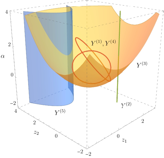
As an illustration, the following figure shows the real part of the incidence variety introduced in Example 5.1 in the article. Our algorithm can compute the projection of each codimension one primary component to the parameter space symbolically or numerically. Section 5 of the paper explains in detail how the algorithm works.
As mentioned above, our symbolic and numerical methods are implemented in julia. Our package \(\verb|PLD.jl|\) can be download here PLD_code.zip. It makes use of HomotopyContinuation.jl (v2.6.4) and Oscar.jl (v0.10.0).
The following Jupyter notebook, which may be downloaded here PLD_notebook.zip, illustrates how to use the main features provided by the package \(\verb|PLD.jl|\).
A Python wrapper for PLD.jl was developed by Tristan Jacquel and can be found at https://github.com/Tracque/PLD-Wrapper.
Database
The following database gives the components of the principal Landau determinant for 23 Feynman diagrams, together with different choices of linear subspaces of the kinematic space, for a total of 114 example diagrams.
For each diagram, we provide: Symanzik polynomials, value of the generic signed Euler characteristic, f-vector of the Newton polytope of the graph polynomial. An additional purpose of this database is to compare the components of the principal Landau determinant with the output given by the \(\verb|cgReduction|\) from HyperInt.
In particular, for each component we indicate:
the method used to compute it, namely, \(\verb|PLD.jl|\) (with symbolic “PLD_sym” or numerical “PLD_num” method) or HyperInt.
the Euler characteristic for generic choices of parameters on the prescribed component.
You can download the complete database by clicking here PLD_database.zip. The notation of the files is as follows \(\verb|NameOfDiagram_internalMasses_externalMasses.txt|\).
If \(\verb|*|\) appears at the end of the file-name, it means that the \(\verb|cgReduction|\) in HyperInt did not terminate on that specific choice of kinematic space.
For further details, we refer to Section 5 and Appendix A in the paper.
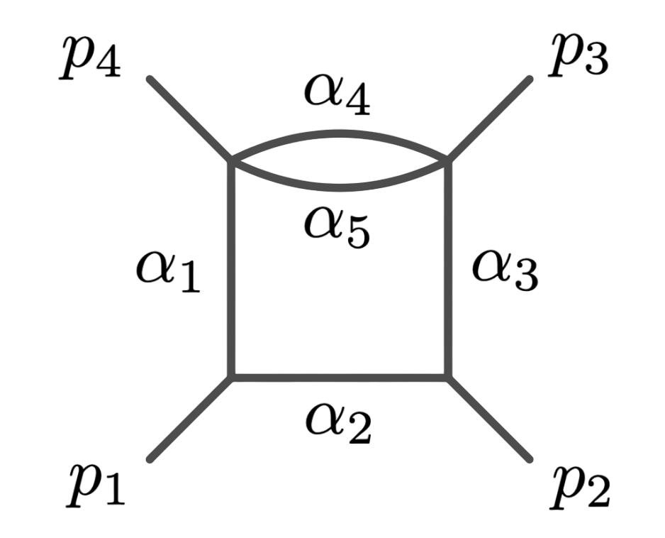
\(G\,=\,\texttt{pentb}\)
|
||
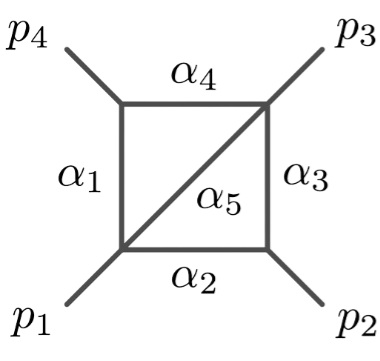
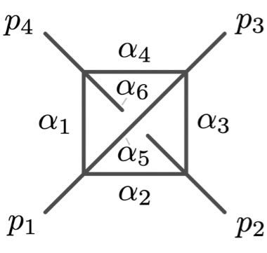
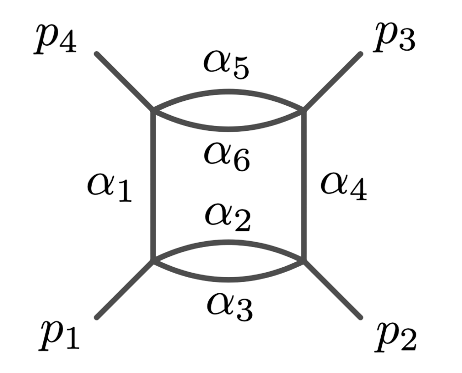
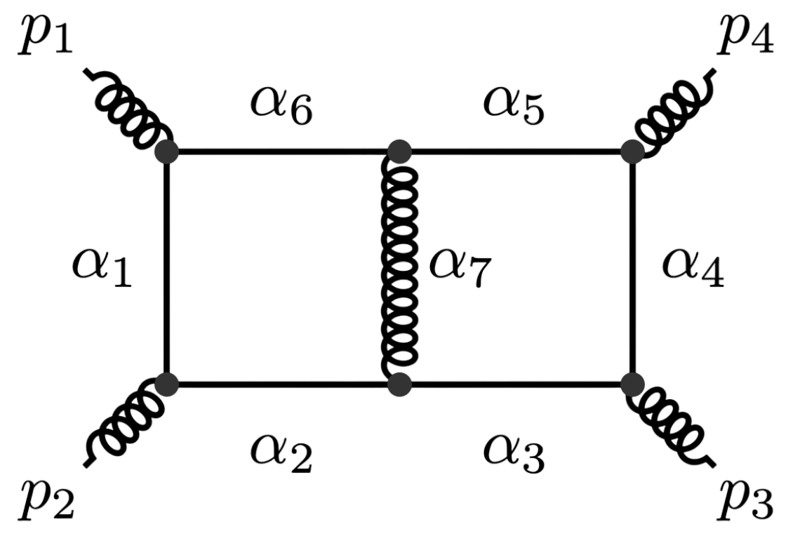
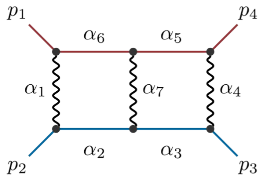
\(G\,=\,\texttt{inner-dbox}\)
|
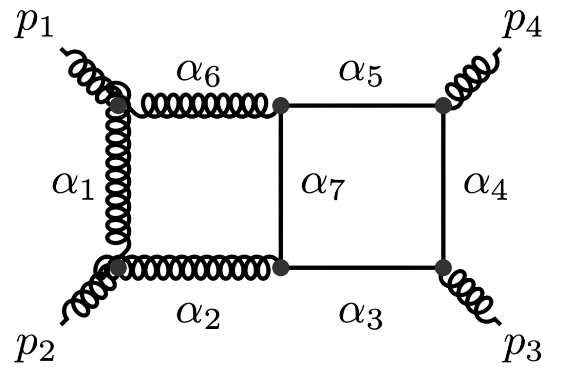
\(G\,=\,\texttt{outer-dbox}\)
|
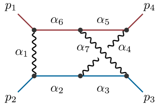
\(G\,=\,\texttt{Hj-npl-dbox}\)
|
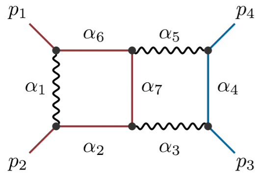
\(G\,=\,\texttt{Bhabha-dbox}\)
|
\(G\,=\,\texttt{Bhabha2-dbox}\)
|
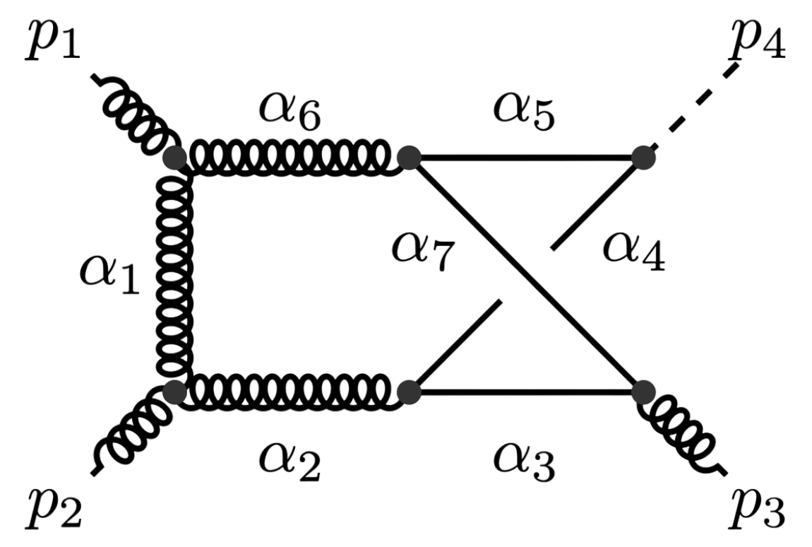
\(G\,=\,\texttt{Bhabha-npl-dbox}\)
|
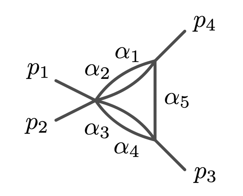
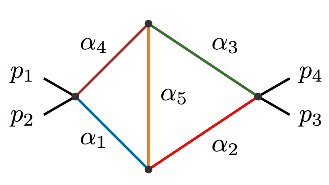
\(G\,=\,\texttt{kite}\)
|
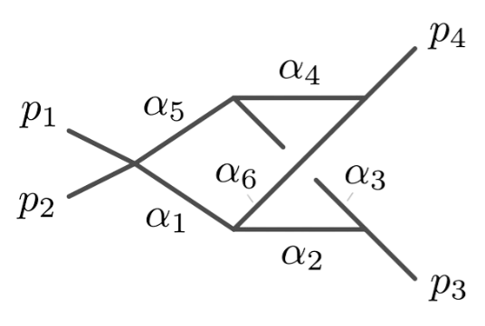
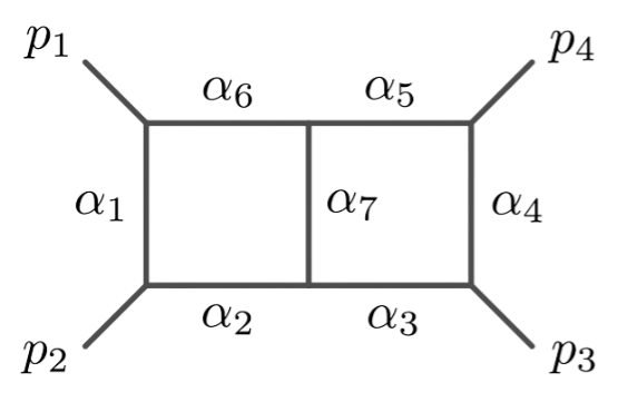
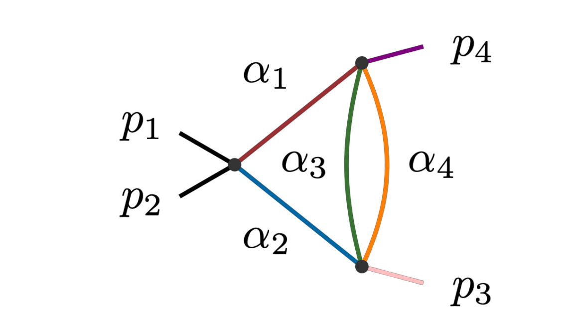
\(G\,=\,\texttt{par}\)
|
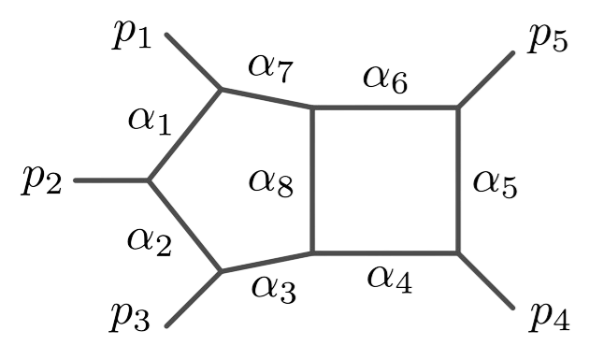
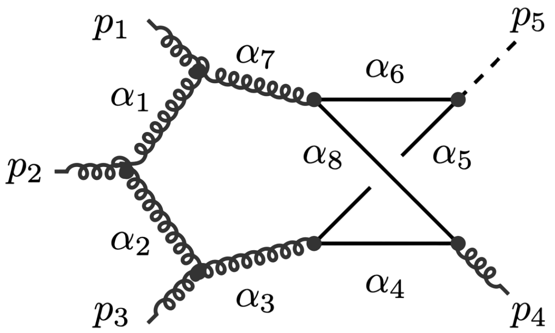
\(G\,=\,\texttt{Hj-npl-pentb}\)
|
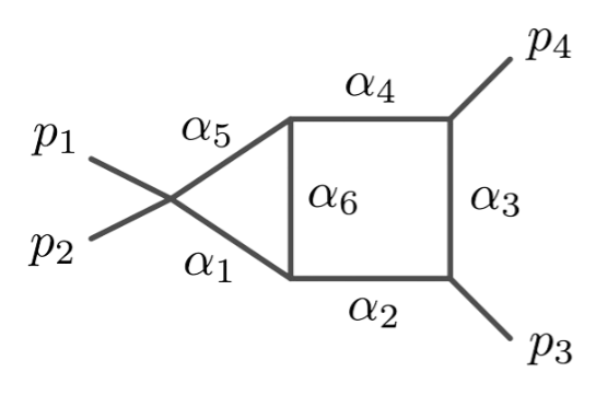
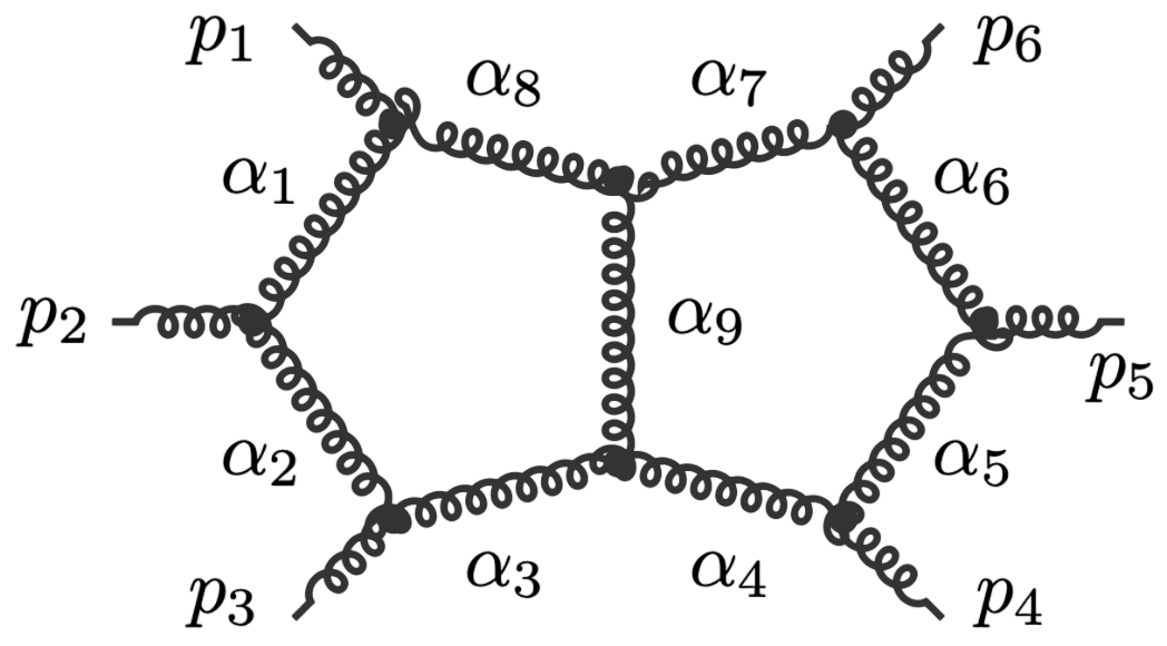
\(G\,=\,\texttt{dpent}\)
|
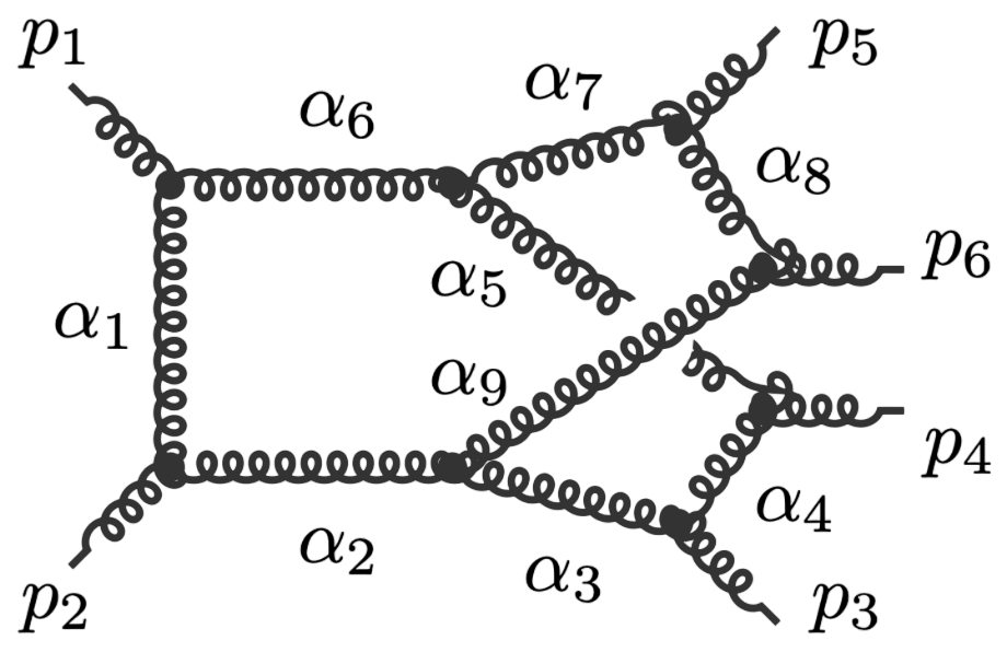
\(G\,=\,\texttt{npl-dpent}\)
|
\(G\,=\,\texttt{npl-dpent2}\)
|
Project page created: 24/11/2023
Project contributors: Claudia Fevola, Sebastian Mizera, Simon Telen
Corresponding author of this page: Claudia Fevola, claudia.fevola@inria.fr
Software used: HomotopyContinuation.jl (Version 2.6.4), Julia (Version 1.8), Oscar (Version 0.10.0)
System setup used: MacBook Pro with macOS Ventura 13.5.1, Chip Apple M2, Memory 16 GB (for running the package on a diagram with no high complexity). For the database: the full computation for one of the simplest diagrams, \(G\,=\,\texttt{inner-dbox}\), took 9.3 minutes, while the most difficult diagram, \(G\,=\,\texttt{npl-dpentb}\), took 63.7 hours on two Intel Xeon E5-2695 v4 CPUs with 18 cores each.
License for code of this project page: MIT License (https://spdx.org/licenses/MIT.html)
License for all other content of this project page: CC BY 4.0 (https://creativecommons.org/licenses/by/4.0/)
Last updated 24/11/2023.