Positive del Pezzo Geometry

This page contains auxiliary files to the paper:

Nick Early, Alheydis Geiger, Marta Panizzut, Bernd Sturmfels, Claudia He Yun: Positive del Pezzo Geometry

arXiv-ID: https://arxiv.org/abs/2306.13604

Abstract: Real, complex, and tropical algebraic geometry join forces in a new branch of mathematical physics called positive geometry. We develop the positive geometry of del Pezzo surfaces and their moduli spaces, viewed as very affine varieties. Their connected components are derived from polyhedral spaces with Weyl group symmetries. We study their canonical forms and scattering amplitudes, and we solve the likelihood equations.

This page is ordered by the same sections as the paper it accompanies. For each section we make the code available that was used to produce examples, stepping stones in proofs or numerical verifications. This data is always labeled according to the corresponding location in the paper.

This page is work in progress, i.e. not all the code and data are available yet. In case of interest in certain computations not yet on this page, please contact us.

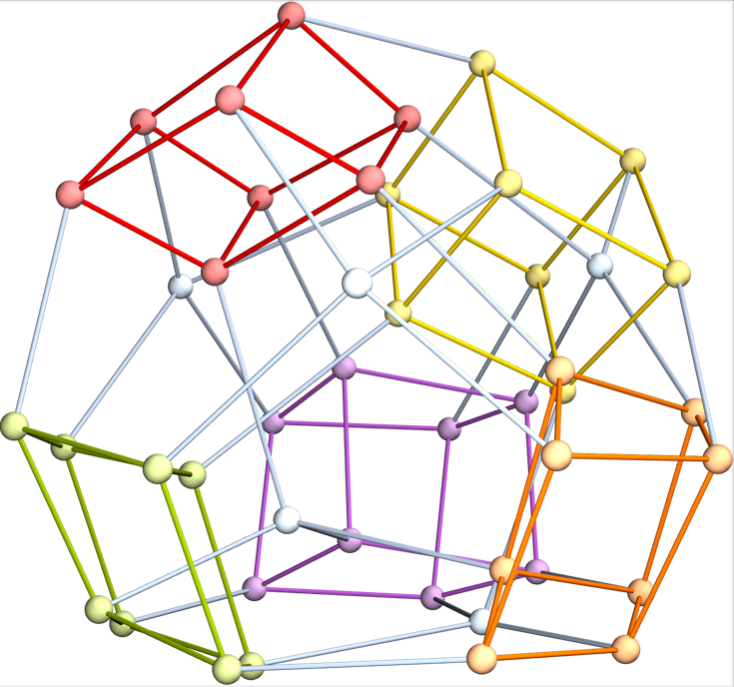
The 15 facets of the E6 pezzotope are displayed here: 10 associahedra and 5 cubes.

Section 2: Blowing up Four Points

We provide code for confirming numerically using the scattering equations formula (CHY) that the scattering amplitude is equal to expression (10). The source code is in \(\verb|Mathematica|\). A notebook with code and explanations can be downloaded here: section2_amplitude.nb

A pdf version of the \(\verb|Mathematica|\) notebook can be viewed here: section2_amplitude.pdf

Code written by: Nick Early and Claudia Yun, 22/06/2023

Software used: Mathematica (Version 13.0)

System setup used: MacBook Pro with macOS Monterey 12.6.1, 2,6 GHz Quad-Core Intel Core i7, Memory 16 GB

Section 3: Polygons

Example 3.2: The source code is in \(\verb|Mathematica|\). A notebook with code and explanations can be downloaded here: Ex3.2.nb

A pdf version of the \(\verb|Mathematica|\) notebook can be downloaded/viewed here: Ex3.2.pdf

Code written by: Claudia Yun, 22/06/2023

Software used: Mathematica (Version 13.0)

System setup used: MacBook Pro with macOS Monterey 12.6.1, 2,6 GHz Quad-Core Intel Core i7, Memory 16 GB

Section 4: Euler Characteristic

Computation of the 2111 strata in \(Y(3,6)\) as displayed in Table 1.

coming soon

Code written by: Claudia Yun, 22/06/2023

Software used: Julia

System setup used: MacBook Pro with macOS Monterey 12.6.1, 2,6 GHz Quad-Core Intel Core i7, Memory 16 GB

Section 5: Numerical Experiments

Experiment 5.1: Code and setup description for computing the Euler Characteristic of \(Y(3,6)\), \(Y(3,7)\)

The source code with brief commentary can be downloaded here:
EulerCharacteristic_Y(3,6).jl
EulerCharacteristic_Y(3,7).jl

Code written by: Alheydis Geiger, 05/04/2023

Software used: Julia (Version 1.9.0), HomotopyContinuation.jl

System setup used: MacBook Pro with macOS Monterey 12.6.6 2,6 GHz Quad-Core Intel Core i7, Memory 16 GB

Experiment 5.2: Code for computing the lower bound of the Euler Characteristic of Y(3,8) as in Theorem 4.1

The source code can be downloaded here: y38.jl

Code written by: Sascha Timme, 21/06/2023

Software used: Julia, HomotopyContinuation.jl (version 2.9.0 )

System setup used: MacBook Pro with M1 Pro Chip and 32 GB RAM

Experiment 5.3: Code on tropical critical points of \(Y(3,6)\).

The source code with brief commentary for the following statements are provided:

There is a unique tropial critical point of multiplicity 32 corresponding to the fibration \(Y(3,6)\to Y(3,5)\): tropical_critical_points_Y(3,6).jl

There tropical critical points with respect to the degeneration of the co-conic condition reveals the boundary of \(Y(3,6)\) in \(X(3,6)\). There are two tropical critical points, one of multiplicity 26 and one of multiplicity 6, which corresponds to \(Y(3,6)= X(3,6)\setminus\mathcal(M)_{0,6}\): tropical_critical_boundary_Y(3,6).jl

Code written by: Alheydis Geiger, 05/04/2023

Software used: Julia (Version 1.9.0), HomotopyContinuation.jl

System setup used: MacBook Pro with macOS Monterey 12.6.6 2,6 GHz Quad-Core Intel Core i7, Memory 16 GB

Experiment 5.4: Code on tropical critical points of \(Y(3,7)\).

The source code with brief commentary for the following statements are provided:
There are 46 tropical critical points corresponding to the fibration \(Y(3,7)\to Y(3,6)\), one of multiplicity 2880 and 45 of multiplicity 16:  tropical_critical_points_Y(3,7).jl
This system is numerically less stable, so it might be necessary to run it a few times to obtain the correct results.

The tropical critical points and their multiplicities can be downloaded here

There tropical critical points with respect to the degeneration of all 7 co-conic conditions reveals the boundary of \(Y(3,7)\) in \(X(3,7)\), by one point of multiplicity 1272, 7 of multiplicity 312 and one of multiplicity 144: tropical_critical_boundary_Y(3,7).jl

The tropical critical points and their multiplicities can be downloaded here

The results are to be read like this: each line is a tropical critical point, the first vector are the coordinates of the tropical Grassmannian, the next vector of 7 coordinates are the tropical values of the co-conic conditions, the last entry of the line is the multiplicity of the tropical critical point.

Code written by: Alheydis Geiger, 05/04/2023

Software used: Julia (Version 1.9.0), HomotopyContinuation.jl

System setup used: MacBook Pro with macOS Monterey 12.6.6 2,6 GHz Quad-Core Intel Core i7, Memory 16 GB

Section 6: Weyl Groups, Roots, and their ML Degrees

group action \(E_6\), \(E_7\)

coming soon

Code written by: Claudia Yun, 22/04/2023

Numerical verification of Prop. 6.1: Code to compute ML degrees of \(E_6\) and \(E_7\)

The source code with explanation can be downloaded here:
MLdegree_E6.jl
MLdegree_E7.jl

Code written by: Alheydis Geiger, 05/04/2023

Software used: Julia (Version 1.9.0), HomotopyContinuation.jl

System setup used: MacBook Pro with macOS Monterey 12.6.6 2,6 GHz Quad-Core Intel Core i7, Memory 16 GB

Experiment 6.3: Code to compute the ML degree of the Yoshida and Göpel parametrization

The source code for the computation of the ML degree of the Yoshida variety can be downloaded here:
MLdegree_Y.jl
The source code for the computation of the log-likelihood function for the computation of the MLdegree of the Yoshida variety  with explanation is available here:
make_eq_for_Y.jl,
together with the data files that are generated by the code and their modifications in re-naming some variables, as explained in the code:
polys_Y (40 polynomials in the 6 variables from \(\mathbb{P}^5\) that give the monomials of the map \(\mathbb{P}^{35}\to\mathbb{P}^{39}\).)
factorised_polys_Y (factorization of the polynomials from above into the 36 different linear factors corresponding to the coordinates of \(\mathbb{P}^{35}\).)
factorised_polys_Yinx (The same polynomials as above, where each of the 36 linear factors is substituted by the corresponding variable x[i] in lexicographic ordering.)
system_for_Y (sum over the 40 polynomials in the 36 variables from above each multiplied by a parameter a[i])

The source code for the computation of the ML degree of the Göpel variety variety with explanation can be downloaded here:
MLdegree_G.jl
matrix_for_G (This file is needed to execute the code in MLdegree_G.jl)
Explanation and the code of the set up is available here:
sytem_for_MLdegree_G.jl

Code written by: Alheydis Geiger, 05/04/2023

Software used: Julia (Version 1.9.0), HomotopyContinuation.jl

System setup used: MacBook Pro with macOS Monterey 12.6.6 2,6 GHz Quad-Core Intel Core i7, Memory 16 GB

Section 8: Combinatorics of Pezzotopes

Clique complex for \(\mathcal{G}(E_6)\), \(\mathcal{G}(E_7)\)

coming soon

Code written by: Nick Early

Theorem 8.2:

coming soon

Code written by: Nick Early

Theorem 8.1: The positive tropical prevarieties of trop(\(\mathcal{Y}\)) and trop(\(\mathcal{G}\)) are simplicial fans with f-vector as in Theorem 8.1.

The \(\verb|Jupyter|\) notebook can be downloded here: E6-Pezzotope.ipynb

The \(\verb|Jupyter|\) notebook can be downloded here: E7-Pezzotope.ipynb

The \(\verb|Jupyter|\) notebook can be viewed here:

The supplementary material to run the computations in the notebook for the \(E_7\) pezzotope can be downloaded here:
gopelprime.jl
E7_raysF2.txt
E7_raysF4.txt
E7_raysF24.txt

The 3 to 6 dimensional cones of the positive tropical Yoshida prevariety as computed in the jupyter notebook can be accessed here:
3dim_cones_E7_pezzotope
4dim_cones_E7_pezzotope
5dim_cones_E7_pezzotope
6dim_cones_E7_pezzotope

Jupyter notebook written by: Marta Panizzut and Alheydis Geiger, 23/06/2023

Software used: Julia (Version 1.9.0),

System setup used: MacBook Pro with macOS Monterey 12.6.6 2,6 GHz Quad-Core Intel Core i7, Memory 16 GB

Section 9: Geometry of Pezzotopes

Proposition 9.1: Code for verification is in \(\verb|Mathematica|\). A notebook with code and explanations can be downloaded here: Prop9.1.nb

A pdf version of the \(\verb|Mathematica|\) notebook can be downloded/viewed here: Prop9.1.pdf

Code written by: Claudia Yun, 23/06/2023

Software used: Mathematica (Version 13.0)

System setup used: MacBook Pro with macOS Monterey 12.6.1, 2,6 GHz Quad-Core Intel Core i7, Memory 16 GB

Theorem 9.4: Data and Code for \(u\)-equations and Gorenstein property of \(E_7\).

coming soon

Section 10: Grassmannians, Positive Geometries, and Beyond

Proposition 10.1: In the proof of the proposition, we claim that for every polygon on \(\mathcal{S}^\circ_6\), we can find six pairwise disjoint lines in \(\mathcal{S}_6\) that are disjoint from the closure of the polygon in \(\mathcal{S}_6\). We verify this claim computationally for the list of polygons from Example 3.2.

The source code is in \(\verb|Mathematica|\). A notebook with code and explanations can be downloaded here: Prop10.1.nb.

A pdf version of the \(\verb|Mathematica|\) notebook can be downloaded/viewed here : Prop10.1.pdf.

Code written by: Claudia Yun, 22/06/2023

Software used: Mathematica (Version 13.0)

System setup used: MacBook Pro with macOS Monterey 12.6.1, 2,6 GHz Quad-Core Intel Core i7, Memory 16 GB

Experiment 10.2

This file provides the rays (as vectors of length 20+1=21) of \(trop_+Y(3,6)\) by modifying the positive tropical Grassmannian with a single vector, due to \(q = p_{123}\cdot p_{345}\cdot p_{156}\cdot p_{246}-p_{234}\cdot p_{456}\cdot p_{126}\cdot p_{135}\). That vector is in position 1 in the list of 15 vectors in the file.

The ordering in each vector is lexicographic: {1,2,3},{1,2,4},{1,2,5},{1,2,6},{1,3,4},{1,3,5},{1,3,6},{1,4,5},{1,4,6},{1,5,6},{2,3,4},{2,3,5},{2,3,6},{2,4,5},{2,4,6},{2,5,6},{3,4,5},{3,4,6},{3,5,6},{4,5,6}.

The file also provides a list of the 2-dimensional cones, which can be used to construct the whole fan.

More information on code and used software on request. Code written by: Nick Early

Theorem 10.3: The bijection between the 34 rays and \(u\)-variables

coming soon

Theorem 10.4

coming soon

Code written by: Nick Early

Project page created: 22/06/2023

Project contributors: Nick Early, Alheydis Geiger, Marta Panizzut, Bernd Sturmfels, Claudia He Yun

Corresponding author of this page: Alheydis Geiger, geiger@mis.mpg.de

License for code of this project page: MIT License (https://spdx.org/licenses/MIT.html)

License for all other content of this project page (text, images, …): CC BY 4.0 (https://creativecommons.org/licenses/by/4.0/)

Last updated 29/11/2023.